Page 1 :
U, , n, , it, , 3b, 3.0 LEARNING OUTCOMES, At the end of this unit, the student will be able to:, Define the terms: primitive or anti derivative and indefinite integrals, Understand integration as inverse process of differentiation, Understand the indefinite integrals as family of curves, Find the integral of simple algebraic functions by substitution, using partial fractions, and by parts, Define definite integral as area of the region bounded by the curve y=f(x), the xaxis and the ordinate x=a and x=b, Apply properties of definite integrals, Apply the definite integral to find consumer surplus-producer surplus, , Integration and Its Application, , 3b.1
Page 2 :
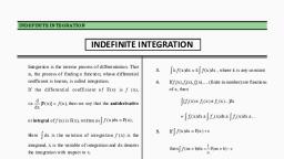
CONCEPT MAP, , 3.1 Introduction:, We already know how to find the differential coefficient (derivative) of a given function. We also, know that the derivative of a function is a function, e.g., the derivative of the function x2 w. r. t., x is the function 2x. Now, we want to find out the function whose derivative is the given function., Suppose the given function is 2x itself. One function whose derivative w.r.t. x is 2x is undoubtedly, x2. But, there could be many other functions such as x2 + 5, x2 + 2, x2 – 1,…,whose derivative w.r.t., x is 2x. In fact, the derivative of x2 + c, where c is an arbitrary constant, w.r.t. x, is 2x., In this section, we shall discuss the process of integration and different methods of integration, along with some applications., The concept of integration is widely used in business and economics. Some of them are, as follows, Marginal and total revenue, cost, and profit;, Capital accumulation over a specified period of time;, Consumer and producer surplus;, , Integral of a function, If, , then we say that the integral or primitive or anti-derivative of f(x) w.r.t. x is, , F(x) and, symbolically, we write, 3b.2, , Applied Mathematics
Page 3 :
In f(x)dx, x is called the variable of integration. The function f(x) is called the integrand. The, symbol stands for the integral., If, , then we also have, , d( F ( x ) C ), f ( x ) , where C is an arbitrary constant, therefore,, dx, , by definition, the integral of f(x) w.r.t. x is F(x) + C, i.e.,, , f (x)dx F(x) C, , The integral of f(x) w.r.t. x is not unique as c can be assigned infinitely many values. It is due, to this indefinite nature of integral, we call it as indefinite integral. If C is assigned the value C1, then, F(x) + C1 is a particular integral of f(x) w.r.t. x., The process of finding integral of a function is called integration., Hence, Integration, as understood above, is nothing but Inverse process of differentiation, Let us consider the following examples:, , We know that derivative of x2 w.r.t. x is 2x and we write, , (x2) = 2x, , Now we may say that anti-derivative (primitive) of 2x w.r.t. x is x2, Further,, , (, , ) = 2x,, , Generalizing this, we may say, , (, , ) = 2x,, , (, , ) = 2x …, , (x2 + C) = 2x which means that anti-derivative of 2x can be, , x2 + 1, x2 + 2 and so on, thereby leading to infinitely many anti-derivatives. Thus, to accommodate, all such anti-derivatives, we may say anti-derivative of 2x is x2 + C where C is an arbitrary constant, or in general called parameter which leads to family of integrals., In general, if, , (F(x) + C) = f(x) then anti-derivative of f(x) w.r.t. x = F(x) + C which is also called, , indefinite integral because C can take any arbitrary value., , Integration and Its Application, , 3b.3
Page 4 :
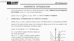
Geometrical Interpretation:, Understanding the integral as family of curves, Consider the curve f(x) = 2x, as discussed earlier, anti-derivative of 2x w.r.t. x is x2 + C = y say, For C = 0, y = x2, For C= 1, y = x2 + 1, For C = -1, y = x2-1 and so on, Thus, we get the family of parabolas whose vertex moves on y axis for different values of, C which can be seen in figure below. This gives the geometrical interpretation of indefinite integral., Thus, we may conclude : indefinite integral gives the family of curves members of which can be, obtained by shifting any one of them parallel to itself., , ÿ, , https://mathinsight.org/indefinite_integral_intuition, , ÿ, , https://mathinsight.org/applet/indefinite_integral_function, , 3b.4, , Applied Mathematics
Page 5 :
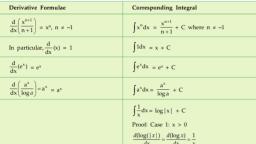
We already know the formulae for the derivatives of many important functions. From these, formulae, we can write down the corresponding formulae (referred to as standard formulae) for the, integrals of these functions, as listed below which will be used to find integrals of other functions., Derivative Formulae, , Corresponding Integral, , d x n 1 , , = xn, n –1, dx n 1 , , In particular,, , , , d, (x) = 1, dx, , x n dx =, , 1dx, , d x, (e ) = ex, dx, , = x + C, , x, , e dx, , d ax , x, , a = ax, dx log a , , , , x n 1, + C where n –1, n 1, , = ex + C, , a x dx =, , ax, + C, log a, , 1, , x dx = log|x| + C, Proof: Case 1: x > 0, , d(log(|x|) d(log x) 1, , , dx, dx, x, Case 2: x < 0, , d(log(|x|) d(log(– x)) 1, 1, , (–1) , dx, dx, –x, x, Some Standard Integrals, we will use (without proof), S. No., , Expression, , 1, , , , 2, , , , Integral, , 1, 2, , x a2, , dx, , 1, 2, , x a, , 2, , dx, , 2, 2, log x x a + C, , 2, 2, log x x a + C, , , , x 2 a 2 dx, , x, a2, 2, 2, x 2 a2 , log x x a + C, 2, 2, , 4, , , , x 2 a 2 dx, , x, a2, 2, 2, x 2 a2 , log x x a, 2, 2, , 5, , x, , 3, , 2, , 1, dx, a2, , Integration and Its Application, , + C, , 1, xa, log, + C, 2, x a, , 3b.5
Page 7 :
c) Let I =, , =, , + C, , d) Let I =, , dx, , =, , dx, , =, , dx, , =, , + C, , =, , + C, , Example 2., The marginal revenue of a company is given by MR = 80+20x+3x2, where x is the number of units, sold for a period. Find the total revenue function R(x) if at x=2, R(x) = 240., Solution: We have, , We find the total revenue function R(x) by integrating, , both sides w.r.t. x, = (80 + 20x + 3x2)dx, ., The constant of integration C can be determined using the initial condition R(x=2) = 240., Hence, 160 + 40 + 8 + C = 240 C = 32., So, the total revenue function is given by, R(x) = 80x + 10x2 + x3 + 32., , Methods of Integration:, In previous section, we discussed integrals of those functions which were readily obtainable from, derivatives of some functions. It was based on inspection, i.e., on the search of a function F whose, derivative is f which led us to the integral., Integration and Its Application, , 3b.7
Page 8 :
However, this method, which depends on inspection, may not work well for many functions., Hence, we need to develop additional techniques or methods for finding the integrals by reducing, them into standard forms. Some important methods are as follows, , 3.2 Integration by substitution, Rule of substitution, where g(x) = t, Proof:, , Note: When we make the substitution g(x) = t, we have, , . Since, the formula established, , above allows us to write g’(x)dx as dt, we may be formally allowed to write equation (1) as g’(x)dx = dt while, working out the solution. Although,, , does not mean dx : dt., , Similar rules may be established such as, where f(x) = t, Consider, Here the integrand is, , for which we do not have direct formula applicable to get the, , integral., If we assume x2 + 1 = t and differentiate, we get 2x =, , Thus, given integral becomes, , which is formally written as 2xdx = dt, , which can be determined using the formula, , =, , + C where n, , + C =, 3b.8, , + C, Applied Mathematics
Page 9 :
putting the value of t we get,, , =, , + C, , Following the above rule, we may also write, , where x = g(t), , Thus, we observe that the given integral f(x) dx can be transformed into another form by, changing the independent variable x to t by substituting x = g (t) and dx = g’(t)dt, Some common substitutions that usually work well are:, Integrand, , Substitution, Put f(x) = t or t2, , f (x), , logx, , Put logx = t or x = et, , fog(x) or f(g(x)), , Put g(x) = t, , f ( x ) m / n, , Put f(x) = tn, , Important Rule: If f(x)dx = F(x) + C then f(ax +b) dx =, , F(ax+b) + C, , Proof: let ax + b = t differentiating we get a dx = dt, Thus, integral becomes f(t), , dt =, , f(t) dt =, , F(ax+b) + C, , Example 3, Evaluate the following:, a), , b) e4-5x dx, , dx, , c) (ax + b)2 dx, , d), , Solution:, a), , dx =, , b) e4-5x dx =, , + C =, , + C, , + C, , c) (ax + b)2dx =, , + C, , d) Let I =, =, , a2x a 2x, , 2x + C, 2, 2, , Integration and Its Application, , 3b.9
Page 11 :
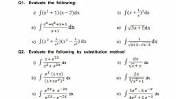
b) Let I =, , dx, , Consider 5 + 4x + x2 = 5 – 4 + 4 + 4x + x2 (by method of completion of squares), = (x + 2)2 + 12, Thus, I =, , = log| x + 2 +, , | + C, , = log| x + 2 +, , | + C, , Example 6, The weekly marginal cost of producing x pairs of tennis shoes is given by, MC = 17 +, , , where C(x) is cost in Rupees. If the fixed costs are, , 2,000 per day, find the cost, , function., Solution: As MC = 17 +, C(x) = MC(x)dx =, , dx = 17x + 200 log|x+1| + C, , Given that, when x = 0, C(x) = 2000, 2000 = 17(0) + 200 log1 + C which gives C = 2000, Hence, C(x) = 17x + 200log|x+1| + 2000, , Exercise 3.1, Q1. Evaluate the following:, i), , ii), , iii), , iv), , v), , vi), , Q2. Evaluate the following by substitution method, i), , iii), , dx, , ii), , dx, , v), , Integration and Its Application, , dx, , iv), , vi), , dx, , dx, , dx, , 3b.11
Page 12 :
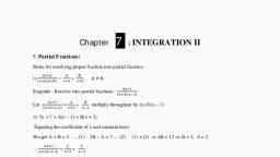
vii), , dx, , ix), , viii), , dx, , Q3. Find i), , ii), , Q4. If the marginal revenue function of a firm in the production of output is MR = 40 – 10x2 where x is, the level of output and total revenue is 120 at 3 units of output, find the total revenue function., Q5. The marginal cost function of producing x units of a product is given by MC =, Find the total cost function and the average cost function, if the fixed cost is, , ., 1000., , (Note: Average Cost Function is obtained by dividing cost function by number of units produced.), Q6. The marginal cost of producing x units of a product is given by MC = x, 3 units is, , . The cost of producing, , 7800. Find the cost function., , 3.3 Integration by Partial Fractions, We know that a rational function is defined as the ratio of two polynomials in the form, , where P(x) and Q(x) are polynomials in x and Q(x) 0., Depending on the degree of P(x) and Q(x), a rational function can be classified as Proper or, Improper., If the degree of P(x) is less than the degree of Q(x), then the rational function is called proper,, otherwise, it is called improper., We may reduce the improper rational functions to the proper rational functions by the process, of long division Thus, if, , is improper, then we may divide P(x) by Q(x). We know that Dividend, , = Divisor X Quotient + Remainder. Thus, P(x) = Q(x) X T(x) + R(x) where degree of R(x) < degree, of Q(x), Therefore,, , =, , +, , = T(x) +, , Example7, Identify the following expressions as Rational Functions. Further classify them as Proper or, Improper. If Improper, express them as sum of a polynomial and proper rational function., a), , 3b.12, , b), , c), , Applied Mathematics
Page 13 :
Solution, a) In, , both numerator and denominator are polynomials, hence, , is a, , rational function, Note : 1 is a constant polynomial of degree 0., As degree of numerator < degree of denominator, hence it is a proper rational function., b) In, , since numerator is not a polynomial, hence, , is not a rational function., , c) In, , both numerator and denominator are polynomials, hence, , is a rational function, As degree of numerator = degree of denominator, hence it is an improper rational function., Consider, , dividing numerator by denominator, we get, x2 + 7x + 12 )x2 + 3x + 2( 1, – x2 + 7x + 12, –4x –10, , Thus,, , x2, , + 3x + 2 = 1 ×, , (x2, , + 7x + 12) + (–4x – 10), +, , = 1 +, , is the required sum of polynomial and proper rational function., , For the purpose of Integration, we shall be considering those rational functions as integrands, whose denominators can be factorised into linear and quadratic factors. In order to evaluate Integral, with integrand, , , where P (x) and Q(x) are polynomials in x and Q(x) 0 and, , is a proper, , rational function. It may be possible to write the integrand as a sum of simpler rational functions, by a method called Partial Fraction Decomposition. Then the integration can be carried out easily, using the already known methods., Here is the list of the types of simpler partial fractions that are to be associated with various kind, of rational functions., , Integration and Its Application, , 3b.13
Page 14 :
S.No., , Type of Rational Function, , 1, , px q, (x a)(x b), , 2, , px 2 qx + c, (x a)(x b)(x c), , Corresponding Partial Fractions Decomposition, A, B, , xa xb, , A, B, C, , , xa xb xc, , px q, , 3, , A, B, , x a ( x a)2, , 2, , (x a), , 4, , px 2 qx + c, (x a)(x b)2, , A, B, C, , , x a x b ( x b)2, , 5, , px 2 qx + c, (x a)(x2 b), , A, Bx C, 2, x a ( x b), , Consider, , =, , +, , . In order to find A and B, we may write px + q = A(x, , + b) + B(x + a). The partial fractions are so designed that this equation turns out to be an identity., Equating coefficients of x and constant terms on both sides, we get p = A + B and q = Ab + Ba,, which can be solved to get A and B. Similarly, we may find A, B and or C for other cases, , Example 8, Express the following as sum of two or more partial fractions and hence integrate, b), , a), , c), , Solution:, a) Let, 1 = A(x + 3) + B(x - 1) = Ax + 3A + Bx – B, 1 = (A + B) x + 3A – B, Comparing coefficients of x and constant terms on both sides we get, A + B = 0 and 3A – B = 1, Solving we get, A =, , and B =, , Let I =, , dx =, , = log|x-1| – log|x+3| + C, 3b.14, , Applied Mathematics
Page 15 :
b) Let, 3x – 2 = A(x – 2)2 + B(x + 1)(x – 2) + C(x + 1), 3x – 2 = A(x2 – 4x + 4) + B(x2 – x – 2) + C(x + 1), = (A + B) x2 + (–4A – B + C) x + 4A – 2B + C, Comparing coefficients of x2, x and constant terms on both sides, we get, A + B = 0, –4A – B + C = 3, 4A – 2B + C = –2, Solving we get A =, , , B =, , Let I =, , , C =, , =, , +, , I =, , 5, , 1, , dx +, 9 (x 2), , + C, , c), , =, , = 1 +, , Now, 4x–10 = A(x–4) + B(x–3) = (A + B)x + (–4A – 3B), A + B = 4, –4A – 3B = -10, Solving we get A = -2, B = 6, So,, , Hence,, , Let I =, , = 1 +, , =, , = x – 2log|x – 3| + 6log|x – 4| + C, , Integration and Its Application, , 3b.15
Page 16 :
Exercise 3.2, Q1. Integrate the following expressions, i), , ii), , iii), , iv), , v), , vi), , vii), , viii), , ix), , x), , xi), , Q2. The marginal revenue function for a firm is given by, , ., , Show that the revenue function is given by, , Q3. Find the total revenue function and demand function, if the marginal revenue function is given by, MR(x) =, , –c, , 3.4 Integration by Parts, Now we will discuss one more method of integration, that can be used in integrating products, of functions., If u and v are any two differentiable functions of a single variable x (say). Then, by the product, rule of differentiation, we have, (u) + u, Integrating both sides w.r.t. x, we get, uv =, , 3b.16, , (u)dx +, , u, , u, , = uv –, , (u)dx, , ...............(i), , Applied Mathematics
Page 17 :
Let u = f(x) and, Then (i) becomes, , = g(x), f(x)g(x), , = f(x) g(x), , –, , f’(x), , g(x), , =f’(x), , If we take f as the first function and g as the second function, then this formula may be stated, as follows:, “The integral of the product of two functions = (first function) × (integral of the second, function) – Integral of the product of (derivative of the first function) and (integral of the second, function)”, There is no particular rule for choosing a function out of the two given functions in the integrand, to be first or second. The one which is easily differentiable may be taken as first function and second, function should be such that its integral is readily available., Usually, the order of first and second functions should be in the order of ILATE functions, where, I, L, A, T, E stand for inverse trigonometric function, logarithmic function, algebraic function,, trigonometrical function, exponential function. This works in most of the situations., , Example 9, Integrate the following:, a), , xe2x, , b) logx, , Solution :, a) Let I =, Assuming x as first function and e2x as second function, and applying by parts, we get, I = x, , + C, , = x., , –, , = x., , ., , + C, , + C, , b) Let I =, Assuming logx as first function and 1 as second function, and applying by parts, we get, I = logx, , + C, = (logx). x -, , + C, , = (logx). x– x + C, Integral of the type:, Let I =, Integration and Its Application, , =, , = I1 + I2 say, 3b.17
Page 18 :
Applying Integration by Parts in I1, we get, I1=, Thus,, , I =, , =, , f(x)e x – f '(x)e x dx e x f '(x)dx C, , f(x)e x – f '(x)e x dx C, , =, , Example 10, Evaluate, a), , b), , c), , d), , Solution :, , Here f(x) = x2 and f’(x) = 2x, , a) Let I =, , b) Let I =, , Here f(x) = logx and f’(x) =, , c) Let I =, Here f(x) =, , and f’(x) =, , d) Let I =, Method 1, Let logx = t, Hence, I =, , 3b.18, , Here f(t) = and f’(t) =, , Applied Mathematics
Page 19 :
Method 2, Let I =, , = I1 + I2, , In I1 =, , Assuming, , as first function and 1 as second function and applying integration by parts, , I1 =, , =, , C, , =, , =, , Thus I =, , + C, , –, , Exercise 3.3, Q1. Integrate the following functions, i) x e2x+3, iv) xlogx, vii) (x2+ 1)logx, , ii) x log(x2 + 1), v) xlog2x, viii) x (log x)2, , iii) x2ex, vi) x2log x, , Q2. Evaluate the following, i), , ii), , iii), , iv), , 3.5 Definite Integral, So far in this topic, we have studied about the indefinite integrals and discussed a few methods, of evaluating these. In this particular section, we shall define definite integral of a function., A definite integral is denoted by, , where a is called the lower limit of the integral and, , b is called the upper limit of the integral., Definite Integral has a fixed value., , Integration and Its Application, , 3b.19
Page 20 :
Area Function, If f(x) is a continuous function defined over [a, b], then we define, , as the area of the, , region bounded by the curve y = f (x), the ordinates x = a and x = b and the x-axis. Let x be a given, point in [a, b]. Then the shaded area in the figure given below is a function of x denoted by A(x), and is called the Area Function. Clearly, A(x) =, , Y= f(x), , First fundamental theorem of Integral Calculus, Theorem 1 : Let f be a continuous function on the closed interval [a, b] and let A (x) be the area, function. Then A’(x) = f (x), for all x (a, b)., , Second fundamental theorem of Integral Calculus, Following theorem enables us to evaluate definite integrals by making use of anti-derivative., Theorem 2 : Let f be continuous function defined on the closed interval [a, b] and F(x) be an antiderivative of f(x). Then, , Note: In, , F(b) – F(a)., , , the function f needs to be continuous in [a, b]., , Further, any anti-derivative works, i.e. If we take the anti-derivative as F(X) + C1 the value of the definite, integral will still turn out to be F(b) – F(a)., , Steps for calculating, (i) Find the indefinite integral, , f(x)dx. Let this be F(x)., , (ii) Evaluate F(b) – F(a) which is equal to the value of, 3b.20, , Applied Mathematics
Page 21 :
Example 11, Evaluate the following definite integrals:, , d), , b), , c), , e), , f), , dx, , Solution :, a), , =, , b), , = log|x+, = log|1+, = log(1+, , |, , - log|0+, )- log1= log(1+, , ), , c), , Consider, x = A(x+4) + B(x+1), x = (A+B)x + 4A+B, comparing coefficients of x and constant terms on both sides, A + B = 1, 4A + B= 0, Solving we get, A =, , I =, , , B =, , 1, 4, 1, 5 4, 8, 4, log x 1 log x 4 1 log log, 3, 3, 3, 2 3, 5, , d), =, =, , =, , =, Integration and Its Application, , 3b.21
Page 22 :
e) Let I =, Consider, =, =, I =, , =, , f) Let I =, , dx, , Consider, =, , = 1+, , Let, 3x–2 = A(x–2) + B(x–1)= (A+B)x + (–2A – B), Comparing, we get 3 = A + B, -2 = -2A – B, Solving we get, A = -1, B = 4, I =, , dx, , = [x – log|x-1| + 4log|x-2|, = 5 – log4 + 4log3 – [3 -log2 + 4log1], = 2 – log2 + 4log3, , Evaluation of Definite Integrals by Substitution, We are aware that one of the important methods for finding the indefinite integral is the method, of substitution., , Steps to evaluate definite integral by the method of substitution, 1. Consider the integral without limits and substitute, y = f (x) or x = g(y) to reduce the given, integral to a known form., 2. Obtain the new limits by putting original limits in the substituted expression., 3. Integrate the new integrand with respect to the new variable without mentioning the, constant of integration., 4. Find the values of answer obtained in (3) at the new limits of integral and find the, difference of the values at the upper and the lower limits., TIP : The step of changing the limits and not re-substituting to get the integral in terms, original variable may save time and avoid tedious calculations., 3b.22, , Applied Mathematics
Page 23 :
Let us understand this, with the help of a few examples., , Example 12, Evaluate the following:, a), , b), , Solution:, a) Let I =, implies 3x2 dx = dt, , Let, , when x = –1, t = 0 and when x = 1, t = 2, I becomes,, I =, , c), Let x + 4 = t dx = dt and x = t – 4, When x = -3, t = 1, when x = 0, t = 4, I becomes,, , dt =, , dt =, , =, , dt, , – 4., 5 4, 2t 2, , 5, , , , 3 4, 4.2 t 2, , 3, , 1, , 1, , 5, , 5, , 3, , 3, , 2. 42 2. 12, 8. 42 8. 12, =, −, −[, −, ], 5, 5, 3, 3, =, =, , Exercise 3.4, Evaluate the following definite integrals, i), , iii), , dx, , dx, , Integration and Its Application, , ii), , iv), , , , 0, , 3, , x, (16 x 4 ), , dx, 3b.23
Page 24 :
v), , dx, , vi), , dx, 1, , vii), , dx, , viii), , ix), , log(1 2x)dx, 0, , x), , dt, , 3.6 Some Properties of Definite Integrals, Here are some important properties of definite integrals. These will be useful in evaluating the, definite integrals more easily., S.N., P1, , Property, , Remark/ Proof, The value of definite integral is independent, of the variable., Proof: Let F(x) be an anti-derivative of f(x), w.r.t. x. Then F(t) will be the anti-derivative, of f(t) w.r.t. t., F (b) – F(a), F (b) – F(a), Hence,, , P2, , Let F(x) be an anti-derivative of f(x) w. r. t. x., Then, by the second fundamental theorem of, calculus, we have, F (b) – F (a), = – [F (a) - F (b)], =, , 3b.24, , Applied Mathematics
Page 25 :
P3, , Let F(x) be anti-derivative of f(x) w. r. t. x., , Then, , = F(b) – F(a), , =[F(b) – F(c)] +[F(c) –F(a)], =, , P4, , Let t = a + b – x. Then dt = – dx., When x = a, t = b and when x = b, t = a., , =, = +, =, , P5, , by P2, by P1, , Let t = a – x. Then dt = – dx., When x = 0, t = a and when x = a, t = 0., , =, = +, =, , P6, , by P2, by P1, , We may write LHS as, Let t = 2a – x. Then dt = – dx., When x = a, t = a and when x = 2a, t = 0, , Integration and Its Application, , 3b.25
Page 26 :
Thus,, =, =, , P7, , if f(2a-x) = f(x), , We know that, , = 0 if f(2a-x) = -f(x), , by P6, Case i) Let f(2a-x) = f(x), , =, Case ii) Let f(2a-x) = -f(x), = 0, , P8, , if f(x) is even, , We may write, , = 0 if f(x) is odd, Note:, , Consider, , and put x = -t which, , A function f(x) is said to be even if, , gives dx = -dt, When, x = -a, t = a and when x = 0, t = 0, , f(-x) = f(x), , eg. f(x) = x2 is even as f(-x), = (-x)2 = x2= f(x), A function f(x) is said to be odd if, f(-x) = - f(x), e.g., f(x) = x3 is odd as f(-x), = (-x)3= -x3= -f(x), 3b.26, , Case i) f(x) is even i.e. f(-x) = f(x). Hence,, = 2, Case ii) f(x) is odd i.e. f(-x) = -f(x). Hence,, = 0, Applied Mathematics
Page 27 :
Let us illustrate the use of these properties with the help of some examples., , Example 13, Evaluate the following definite integrals, a), , b), , Solution: a) Let I =, (x 2),, We know that x 2 , (x 2),, , I=, , x2, x 2, by P3, , =, = -, , +, , =-, , +, , = 2 + 2 = 4, b) Let I =, Let, , = 0 gives x = -1, 0, 1, , Clearly,, , As 0, 1 (-1, 2), by P3, , We may w rite, I =, , =, =, =, , -, , =, , Integration and Its Application, , 3b.27
Page 28 :
Example 14, , Evaluate, , Solution, , dx, , Let I =, , ……..(1), , Here a = -1, b = 1, Replacing x by a + b - x i.e. 0 - x, we get, I=, , by P4, , I =, , …….(2), , Adding (1) and (2), we get, 2I =, 2I =, 2I = x, 2I = 1 – (-1) = 2, I = 1, , Example 15, , Evaluate, , Solution, , Let I =, , ……..(1), , Replacing x by 1-x, we get, I =, , 1, , ∫0, , log (1− ), log (1−x) + log (1−(1− )), , I =, , dx, , by P3, , …….(2), , Adding (1) and (2), we get, 2I =, 3b.28, , Applied Mathematics
Page 29 :
2I =, 2I = x, 2I = 1, I =, , Example 16, , dx, , Let I =, , ……..(1), , Here a = 1, b = 3, Replacing x by a + b - x i.e. 4 - x, we get, I =, , dx by P4, , I =, , …….(2), , Adding (1) and (2), we get, 2I =, , 2I =, 2I = x, 2I = 3 – 1 = 2 gives I = 1, , Exercise 3.5, Q1. Evaluate the following definite integrals:, i), , where f(x) =, , ii), , Integration and Its Application, , iii), , 3b.29
Page 30 :
iv), , v), , vi), , vii), , viii), , x), , dx, , dx, , ix), , dx, , dx, , xi), , xii), , Q2. Evaluate, , where [.] denotes Greatest integer function, , 3.7 CONSUMERS’ SURPLUS AND PRODUCERS’ SURPLUS, CONSUMERS’ SURPLUS (CS), Let us first recall Demand Curve, What Is the Demand Curve?, The demand curve is a graphical representation of the relationship between the price of a good, or service and the quantity demanded for a given period of time. In a typical representation, the, price will appear on the left vertical axis, the quantity demanded on the horizontal axis., , Understanding the Demand Curve, We know that as per the law of demand as the price of a given commodity increases, the, quantity demanded decreases, all else being equal. Thus, the demand curve will move downward, from the left to the right as shown in the figure given below:, , 3b.30, , Applied Mathematics
Page 31 :
Let us assume that the prevailing market price is p0. Let the quantity of commodity sold at price, po, as determined by demand curve be xo as shown in figure below., , A consumer surplus happens when the price that consumers pay for a product or service is less, than the price, they’re willing to pay. It is the measure of the additional benefit that consumers, receive because they are paying less for something than what they were willing to pay. Consumers’, surplus always increases as the price of a good falls and decreases as the price of a good rises., However, there are buyers who would be willing to pay a price higher than p0. These buyers will, gain from the fact that the prevailing market price is only p0. This gain is called Consumers’ Surplus., It is represented by the area below the demand curve p = f(x) and above the line p = p0., , Thus, Consumers’ Surplus, CS = [Total area under the demand function bounded by x = 0, x =, x0 and x-axis – Area of the rectangle OAPB], CS =, , – p 0x 0, , Example 17, Find the consumers’ surplus for the demand function p = 25 - x - x2 when p0 = 19., Solution: Given that, the demand function is p = 25 - x - x2, p0 = 19, 19 = 25 - x - x2, x2 + x – 6 = 0, , Integration and Its Application, , 3b.31
Page 32 :
(x + 3) (x – 2) = 0, x = 2 (or) x = -3, x0 = 2 [demand cannot be negative], p0x0 = 19 x 2 = 38, CS =, , – 38 = 25x –, , x3, –, 3, , Example 18, The demand function for a commodity is p =, , ., , Find the consumers’ surplus when the prevailing market price is 5., Solution: Given that, Demand function, p =, , p0 = 5 5 =, , x = 1 i.e. x0 = 1, , p 0x 0 = 5, CS =, = 10 [log(x + 1)], , – p 0x 0, –5., , = 10[log 2 – log 1] -5 = 10 log2 - 5, , PRODUCERS’ SURPLUS (PS), What Is the Supply Curve?, The supply curve is a graphical representation of the relationship between the price of a good, or service and the quantity supplied for a given period of time. In a typical representation, the price, will appear on the left vertical axis, the quantity supplied on the horizontal axis., Thus, a supply curve for a commodity shows the quantity of the commodity that will be brought, into the market at any given price p., As the price of a given commodity increases, the quantity supplied increases (all else being equal)., , 3b.32, , Applied Mathematics
Page 33 :
Suppose the prevailing market price is p0. At this price a quantity x0 of the commodity, determined, by the supply curve, will be offered to buyers as shown in figure below., , However, there are producers who are willing to supply the commodity at a price lower than, p0. All such producers will gain from the fact that the prevailing market price is only p0. This gain, is called ‘Producers’ Surplus’., It is represented by the area above the supply curve p = g(x) and below the line p = p0 as shaded, in figure below., , Thus, Producers’ Surplus, PS = [Area of the whole rectangle OAPB - Area under the supply, curve bounded by x = 0, x = x0 and x - axis], i.e. PS = p0x0 –, , Example 19, The supply function for a commodity is p = x2 + 4x + 5 where x denotes supply. Find the, producers’ surplus when the price is 10., Solution: Given that, Supply function, p = x2 + 4x + 5, For p0 = 10, we have 10 = x2 + 4x + 5 x2 + 4x - 5 = 0, (x + 5) (x - 1) = 0 x = -5 or x = 1, Since supply cannot be negative, x = -5 is not possible., x = 1, As p0 = 10 and x0 = 1 ?p0x0 = 10, 1, , Producers’ Surplus, PS = p0x0 –, = 10 – [ +, , Integration and Its Application, , ] = 10 – [, , = 10 –, , (x, 0, , 2, , + 4x + 5)dx, , + 2 + 5] =, , 3b.33
Page 34 :
Equilibrium Price and Quantity, On a graph, the point where the supply curve P = S(Q) and the demand curve P = D(Q), intersect is the equilibrium. The equilibrium price is the price where the amount of the product that, consumers want to buy (quantity demanded) is equal to the amount producers want to sell (quantity, supplied). This mutually desired quantity is called the equilibrium quantity., , ef, , Refer to following link for further details, ÿ, , https://www.youtube.com/watch?v=W5nHpAn6FvQ&t=20s, , Steps to find equilibrium price and quantity, 1) Solve for the demand function and the supply function in terms of Price (p)., 2) Equate xs (quantity supplied) to xd (quantity demanded). The equations will be in terms, of price (p), 3) Solve for p, the value so obtained will be called equilibrium price., 4) Substitute equilibrium price into either demand or supply function (or both—but most, times it will be easier to put into supply function) and solve for x, which will give required, equilibrium quantity., , Example 20, Suppose that demand is given by the equation xd=500 – 50P, where xd is quantity demanded, and, P is the price of the good. Supply is described by the equation xs= 50 + 25P where xs is quantity, supplied. What is the equilibrium price and quantity?, Solution : 20 We know that, for equilibrium price xd = xs, hence we get, 500-50P = 50+25P, i.e. 450 = 75P which gives P = 6, putting P = 6 in xd = 500 – 50P we get x = 500 - 50(6) = 200, , 3b.34, , Applied Mathematics
Page 35 :
Exercise 3.6, 1), 2), 3), 4), 5), 6), 7), , If the demand function is p = 35 - 2x - x2 and the demand x0 is 3, find the consumers’ surplus., If the demand function for a commodity is p = 25- x2, find the consumers’ surplus for p0 = 9., The demand function for a commodity is p = 10 - 2x. Find the consumers’ surplus for (i) p = 2 (ii), p = 6., The demand function for a commodity is p = 80 - 3x - x2. Find the consumers’ surplus for p = 40., If the supply function is p = 3x2 + 10 and x0 = 4, find the producers’ surplus., If the supply function is p = 4 - 5x + x2, find the producers’ surplus when the price is 18., If the demand and supply curve for computers is D = 100 - 6P, S = 28 + 3P respectively where P, is the price of computers, what is the quantity of computers bought and sold at equilibrium?, , CASE BASED QUESTION, Question: The second new species named Puntius euspilurus is an edible freshwater fish found, in the Mananthavady river in Wayanad. The epithet euspilurus is a Greek word referring to the, distinct black spot on the caudal fin. The slender bodied fish prefers fast flowing, shallow and clear, waters and occurs only in unpolluted areas. It appears in great numbers in paddy fields during the, onset of the Southwest monsoon., , Suppose that the supply schedule of this Fish is given in the table below which follows a linear, relationship between price and quantity supplied., PRICE P PER KG (IN, , ), , QUANTITY (X) OF FISH SUPPLIED (IN KG), , 25, , 800, , 20, , 700, , 15, , 600, , 10, , 500, , 5, , 400, , Suppose that this Fish can be sold only in the Kerala. The Kerala demand schedule for this Fish is, as follows and there is a linear relationship between price and quantity demanded., PRICE(p) PER KG (IN, , ), , QUANTITY (x) OF FISH DEMANDED (IN KG), , 25, , 200, , 20, , 400, , 15, , 600, , 10, , 800, , 5, , 1000, , Integration and Its Application, , 3b.35
Page 36 :
Q1. Which of the following represents the Price (p) - supply(x) relationship?, x, 20, x, c) p = -15 +, 20, , x, 20, x, d) p = 15 20, , a) p = 65 -, , b) p= 65 +, , Q2. The equation of demand curve can be given by, x, 40, x, c) p = 20 –, 40, , x, 40, x, d) p = 20 +, 40, , a) p = 30 –, , b) p = 30 +, , Q3. The value of x at equilibrium is, a) 1400/3, b) 600, c) 15, d) 200/3, Q4. The equilibrium price is, a) 400, b) 20, c) 600, d) 15, Q5. The consumers’ surplus at equilibrium price is, a) 18009, b) 13500, c) 9000, d) 4500, , Miscellaneous Exercise, Q1. Integrate the following, i) x3, iii), v), , ii), dx, , iv), , dx, , vi), , dx, dx, , (1 x)log x dx, , Q2. Evaluate the following, i), , ii), , iii), , iv), , v), , vi), , Q3. Show that, , dx =, , dx, , + 2x + C, , Q4. A firm finds that quantity demanded and quantity supplied are 30 units when market price is 8 per, unit. Further, if price is increased to 12 per unit, demand reduces to 0 and at a price of 5 per, unit, the firm is not willing to produce. Assuming the linear relationship between price and quantity, in both cases, find the demand function, supply function and consumers’ surplus and producers’, surplus at equilibrium price., 3b.36, , Applied Mathematics
Page 37 :
SUMMARY, This reverse process of differentiation is termed as Integration., A function f which on differentiating gives f’ is called anti-derivative (or primitive) of the function., If, , (, , ) = f(x) then anti-derivative of f(x) = F(x) + C which is also called indefinite integral, , because C can take any arbitrary value., Formulae of Integration, =, , + C where n, , =x +C, = ex + C, =, , + C, , = log|x| + C, , dx = log(x +, , )+ C, , dx = log(x +, , )+ C, , =, , +, , log |x +, , –, , dx =, , dx =, , Type of Rational Function, , log |x +, , + C, , + C, , + C, , + C, , Corresponding Partial Fractions Decomposition, +, , +, , Integration and Its Application, , +, , C, xc, 3b.37
Page 38 :
+, , +, , +, , +, , INTEGRATION BY PARTS:, , f(x)g(x), , = f(x) g(x), , A definite integral is denoted by, , -, , f’(x), ’(x), , g(x), , where a is called the lower limit of the integral and, , b is called the upper limit of the integral., Definite Integral has a fixed value., Let f be continuous function defined on the closed interval [a, b] and F be an anti-derivative of, f. Then,, , F(b) – F(a)., , Properties of Definite Integral, , where, , 3b.38, , Applied Mathematics
Page 39 :
, , 2a, , 0, , , f(x)dx 2, , , , , a, , 0, , f(x)dx, , if f(2a-x) = f(x), = 0 if f(2a-x) = -f(x), , a, , , f(x)dx 2, a, , , , , , , a, , 0, , f(x)dx, , if f(x) is even, = 0 if f(x) is odd, , Cost Function, C(x) = MC(x)dx where MC is Marginal Cost, Revenue Function, R(x) = MR(x)dx where MR is Marginal Revenue, Consumers’ Surplus, CS =, , – p0x0 where f(x) is the demand curve, , Producers’ Surplus, PS = p0x0 -, , where g(x) is the supply curve, , The equilibrium price is the price where the amount of the product that consumers want to buy, (quantity demanded) is equal to the amount producers want to sell (quantity supplied). This, mutually desired amount is called the equilibrium quantity., , ANSWERS, EXERCISE 3.1, Q1, , i), , iii), , v), , Q2, , + C, , + C, , iii), , + C, , vii) log |, , ix), , Integration and Its Application, , +C, , vi), , + C, , v), , + C, , iv), , +C, , i), , ii), , ii) 2log (, , iv), , + C, , + C, , +, , vi), , viii), , + C, , + 1) + C, , + C, , –x 7, log 4e x 5e –x C, 8 8, + C, , + C, , 3b.39
Page 40 :
Q3., , i) log |x +, , i), , | - 2, , log | x +, , Q4. R(x) = 40x -, , + C, , +, , |+ C, , + 90, , Q5. C(x) =, , + 950, Average Cost =, , Q6., , –, , +, , EXERCISE 3.2, Q1, , i), , + C, , ii) -x +, , + C, , ii), , + C, , iv) log|logx – 2| - log|logx – 1| + C, , v), , + C, , vi) -x – e-x + log |ex + 1| + c, vii), , + C, , viii), , +C, , ix), , +C, , x), , xi) log|x| –, , + C, , +C, , EXERCISE 3.3, Q1, , i), iii), v), vii), , 3b.40, , - 2x, , + C, + 2, , ii), , + C, , x2, x2, log2x –, C, 2, 4, , iv), vi), , –x + C, , viii), , x2 1, 2, , + C, + C, + C, + C, , Applied Mathematics
Page 41 :
Q2, , i), , + C, , iii), , ii), , + C, , + C, , iv) x[loglogx -, , ]+ C, , EXERCISE 3.4, i) log2, , ii) log2, , iii), , iv), , v), , vi), , vii) log2, , ix) 10 +, , viii), , 3, 2, [(1 e) 2 2 2], 3, , 3, log3 – 1, 2, , x) log, , log3, , 4, 3, , EXERCISE 3.5, Q1., , i), , ii), , iii) 4, , iv) 2, , v), , vi) 20, , vii) 2, , viii) 2log2, , ix), , x), , xi) 0, , 2 2 2log | 1 2 |, , xii), , Q2. 1, , EXERCISE 3.6, 1., , 27, , 3., , i) 16, , 2., ii) 4, , 5. 128, , 4., , 6., , 7. 52, Integration and Its Application, , 3b.41
Page 42 :
CASE BASED QUESTION, 1. c, , 2. a, , 3. b, , 4. d, , 5. d, , MISCELLANEOUS EXERCISE, Q1., , i), , iii), , + C, , log |, , v) log, Q2., , i), , +, , +, , ii), , | +C, , + C, , + 3log2 – log 3, , + C, , iv), , + C, , vi), , log x - x -, , + C, , ii) 6, , iii) 0, , iv), , v) 1, , vi), , 2 2, 3, , Q4. Demand Function: p = 12 Supply Function: p =, , + 5, , Consumers’ Surplus = 60, Producers’ Surplus = 45, , , 3b.42, , Applied Mathematics