Page 1 :
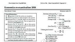
NON FOCUS AREA - MICRO ECONOMICS, CHAPTER – 1, INTRODUCTION, Production Possibility Curve, Production possibility frontier.The curve obtained by joining the alternative combinations of, two goods produced in the economy using full employment of resources and constant, technology., Production possibilities, , Good 1, , Good 2, , B, , 0, , 15, , C, , 1, , 14, , G, , 2, , 12, , H, , 3, , 9, , I, , 4, , 5, , J, , 5, , 0
Page 2 :
Point G – Under utilisation of resources., Point H – Full employment of resources., Point I – Growth of resources., , Positive economics, , Normative economics, , Answer the question 'what is?', , Answer the question 'what ought to be?', , Explains how a mechanism functions Explains whether the mechanism desirable or not, , No value judgment, , Value judgment is possible, , CHAPTER – 2, THEORY OF CONSUMER BEHAVIOUR, Price elasticity of demand:Price elasticity of demand may be defined as the degree of responsiveness in, quantity demanded of the good due to change in it’s price., percentage change in quantity demanded of the good, Price elasticity of demand, Ed =, percentage change in price of the good, Types or degrees of price elasticity of demand:- Five types., 1. Elastic demand, 2. Inelastic demand, 3. Unitary elastic demand, 4. Perfectly inelastic demand, 5. Perfectly elastic demand, 1. Elastic demand:* Percentage change in quantity demanded is greater, than percentage change in price of the good., * Value of elasticity is grater than one or unity. ( Ed > 1), 2. Inelastic demand:* Percentage change in quantity demanded is less, than percentage change in price of the good., * Value of elasticity is less than one or unity. ( Ed < 1)
Page 3 :
3. Unitary elastic demand:* Percentage change in quantity demanded is equal, to percentage change in price of the good., * Value of elasticity is equal to one or unity. ( Ed = 1), * Demand curve is rectangular hyperbola., , price, P1, P, 0, , 4. Perfectly inelastic demand:* Percentage change in quantity demanded is constant, at what may be the level of price of the good., * Value of elasticity is zero. ( Ed =0), * Demand curve is vertical line to X axis., , price, P1, P, 0, , 5. Perfectly elastic demand:* No change in price of the good. But, the quantity demanded of the good changes., * Value of elasticity is infinity. ( Ed = ꝏ), * Demand curve is horizontal straight line to X axis., , D, Q1 Q demand, D, , Q demand, , price, p, D, 0, , Q, , Q1 demand, , Constant elasticity of demand:1. Unitary elastic demand (Ed = 1), 2. Perfectly inelastic demand (Ed = 0), 3. Perfectly elastic demand (Ed = ꝏ), Methods of Measurement of Price elasticity of demand:1. Percentage method ( Proportionate method), 2. Geometric method ( Point method), 3. Expenditure method, 1. Percentage method:- By percentage method, price elasticity of demand is;, percentage change in quantity demanded of the good, Ed =, percentage change in price of the good, For example, suppose 10% increase in price of a good is resulted to 30% fall in quantity, demanded of that good. Then;, Ed = 30/10 = 3. Demand is elastic because Ed > 1., The following formula is also used for the calculation of price elasticity of demand., ΔQ P, Ed =, X, ΔP Q, Where; Ed = price elasticity of demand,, P = initial price of the good, Q= initial quantity demanded, Δ Q = change in quantity demanded.(Q1 – Q). Q1 = second quantity demanded, Δ P = change in price. ( P1 – P) . P1= second price of the good., For example, the price of good X increases from rupees 20 to 40. As a result it’s quantity demanded, decreased from 100 units to 50 units. Then;, ΔQ, Ed =, , P, X, , ΔP, , Q, , P = 20
Page 4 :
P1 = 40, Δ P = P1 – P = 40 – 20 = 20, Q = 100, Q1 = 50, Δ Q = Q1 – Q = 50 – 100 = -50, -50, Ed =, , 20, X, 20 100, -50, , =, 100, = - 0.5 Inelastic demand because Ed < 1, (Not consider the negative sign of the answer. It shows only the negative relation between price and, quantity demanded of the good. So the value of elasticity is 0.5), 2.Geometric method of measurement of price elasticity of demand, Geometric method measures elasticity at a point on a linear demand curve., The following formula is used for the calculation of elasticity at a point on the linear demand curve, -bP, p= price, Ed =, b = slope of demand curve., Q, Q = quantity demanded, Using this formula, the five values of elasticity can be measured at different points on a linear, demand curve as follows., *At horizontal intercept ( p=0) ; Ed = 0, *At vertical intercept ( p = a/b ) ; Ed = ꝏ, *At mid point of the curve ( p = a/2b ) : Ed = 1, *At any point between mid point & horizontal intercept ( p < a/2b ) ; Ed < 1, *At any point between mid point & vertical intercept ( p > a/2b ) ; Ed > 1, , Q. Suppose a demand function is d(p) = 10 – 3p. Calculate price elasticity of demand at price, rupees 5/3.
Page 5 :
-bP, Ed =, Q, , d(p) = 10 - 3p, p = 5/3, b=3, Q = 10 – 3 X 5/3 = 10 – 5 = 5, , Ed = - 3 X 5/3, 5, = - 5/5 = -1 . Unitary elastic demand ( Ed = 1 ), Similarly, another way is used for the calculation of price elasticity of demand by the, geometric method. The method is as follows., , 3. Expenditure method of measurement of elasticity:This method measures three degrees of elasticity of demand., a) Inelastic demand (Ed<1):* price and expenditure are moving in same direction., * Price increases the expenditure also increases. (Due to % fall in demand is less than % increase in, price), * Price falls the expenditure also falls. (Due to % increase in demand is less than % fall in price), b) Elastic demand (Ed>1):* Price and expenditure are moving in opposite direction., * Price falls but, expenditure increases. (Due to % increase in demand is higher than % fall in, demand., * Price increases but, expenditure falls. (Due to % fall in demand is higher than % increase in price), c) Unitary elastic demand (Ed=1), * Price changes (increases or decreases) but expenditure does not change. (Due to % change in, demand is equal to the % change in price)
Page 6 :
Determinants of price elasticity of demand:1. Nature of the goods :- The demand for necessary good is inelastic. But the demand for luxury, good is elastic., 2. Availability of substitute goods :- The demand for the goods with substitute is elastic. But the, demand for the goods without substitute is inelastic., 3. Level of income:- The demand for the goods by rich people is inelastic. But the demand for the, same goods by poor people is elastic., 4. Price level :- The demand for the goods at low price level is inelastic. But the demand for the, goods at high price level is elastic., CHAPTER – 3, PRODUCTION & COST, Returns to scale:Returns to scale represent a long run production function. Returns to scale explain the, change in output when all inputs are changing in the same proportion. There are three types of, returns to scale in the production., 1. Increasing returns to scale(I R S), 2. Constant returns to scale (C R S), 3. Diminishing returns to scale (D R S), 1. IRS:- In this case, output increases at a more than proportionate increase in inputs. For example,, 20% increase in inputs resulted to 40% increase in output. Symbolically, I R S can be represented, as;, q = f (X1,X2), f (t. X1, t. X2) > t. f(X1,X2) where, t = proportion of change in inputs., 2. C R S:- In this case, the output increases at an equal proportionate increase in inputs. For, example, 20% increase in inputs resulted to 20% increase in output. Symbolically, C R S is;, f (t. X1, t. X2) = t. f(X1,X2), 3. D R S:- In this case, the output increases at a less than proportionate increase in inputs. For, example, 20% increase in inputs resulted to 10% increase in output. Symbolically, C R S is;, f (t. X1, t. X2) < t. f(X1,X2), Differences between variable proportions & returns to scale:Variable proportions, Returns to scale, A short run production function, , A long run production function, , One input is variable, other input is fixed, , All inputs are variable in same proportions, , Three forms of changes in output – increasing, returns, diminishing returns, negative returns, , Three forms of changes in output – increasing, returns, constant returns, diminishing returns, , Cobb-Douglas production function:This production function has the form;, , In this production function,
Page 7 :
Q. Suppose q= 5L².K² is a production function. Calculate maximum output when L=10 and K=5., q= 5L².K², q= 5X 10² X 5², q= 5 X 100 X 25, q= 500 X 25, q= 12500, ASSIGNMENT:1. Let the production of a firm be q=5L¹/².K¹/². Find out the maximum possible output that the firm, can produce with 100 units of L and 25 units of K., 2. Let the production function of a firm be q=2L².K². Find out the maximum possible output that the, firm can produce with 3 units of L and 4 units of K. What is the maximum possible output that the, firm can produce with zero units of L and 10 units of K?, 3. Find out the maximum possible output for a firm with zero units of L and 20 units of K when it’s, production function is q = 5L + 2K., Long run cost:In the long run the firm uses only variable inputs. So the firm has only variable cost in, the long run. That means the firm has no fixed cost in the long run. Firm’s total cost is it’s variable, cost. In the long run the firm has two types of costs. They are, 1. Long run average cost (L R A C), 2. Long run marginal cost (L R M C), 1. L R A C:LRAC=TC/ q, 2. L R M C:LRMC=ΔTC/Δq, L R M C = T C n – T C n-1, Relationship between L R A C & L R M C:L R A C & L R M C curves have ‘U’ shape., cost, LRMC, LRAC, E, , O, Q quantity, a) L R A C falls when L R M C is below L R A C, b) L R A C is minimum when L R A C = L R M C., c) L R A C increases when L R M C is above L R A C., L R A C curve has ‘U’ shape due to returns to scale., * Initially L R A C falls due to I R S (Increasing Returns to Scale), * L R A C is minimum due to C R S (Constant Returns to Scale)., * L R A C increases due to D R S (Diminishing Returns to Scale).
Page 8 :
CHAPTER - 4, THEORY OF FIRM UNDER PERFECT COMPETITION, Determinants of Supply:1. Price of the good. ( Positive relation to supply), 2. Input prices. (Negative relation to supply), 3. State of technology.( Positive relation to supply), 4. Unit tax.(Negative relation to supply), 5. Cost of production. (Negative relation to supply), Market supply schedule & Market supply curve:The horizontal summation of individual supply schedules is the market supply schedule., , The horizontal summation of individual supply curves is the market supply curve., , Changes in supply:1. Movement along the supply curve, (a) expansion of supply, (b) contraction of supply, 2. Movement of the supply curve
Page 9 :
(a) increase in supply, (b) decrease in supply, 1. Movement along the supply curve, Expansion of supply, Increase in supply due to increase in price., Contraction of supply, Decrease in supply due to decrease in price., , 2. Movement of the supply curve(Shifts in supply):A. increase in supply : Rightward shift of supply curve., Causes: *Development of technology *Fall in cost of production *Input price falls *Unit tax rate, falls., Price, , S, , S1, , supply, , B. decrease in supply : Leftward shift of supply curve .
Page 10 :
Causes - *Poor technology *Rise in cost of production *Input price rises *Unit tax rises, , Price, , S1, , S, , supply, Methods of Measurement of Price elasticity of supply:1. Percentage method ( Proportionate method), 2. Geometric method., 1. Percentage method:- By percentage method, price elasticity of supply is;, percentage change in quantity supplied of the good, Es =, percentage change in price of the good, For example, suppose 10% increase in price of a good is resulted to 30% increase in quantity, supplied of that good. Then;, Es = 30/10 = 3. Demand is elastic because Ed > 1., The following formula is also used for the calculation of elasticity of supply., ΔQ P, Ed =, X, ΔP Q, Where; Es = price elasticity of supply,, P = initial price of the good, Q= initial quantity supplied, Δ Q = change in quantity supplied.(Q1 – Q). Q1 = second quantity supplied., Δ P = change in price. ( P1 – P) . P1= second price of the good., For example, the price of good X increases from rupees 20 to 40. As a result it’s quantity supplied, increased from 100 units to 150 units. Then;, ΔQ, Es =, , X, ΔP, , 50, Es =, , P, Q, , 20, X, 20 100, , P = 20, P1 = 40, Δ P = P1 – P = 40 – 20 = 20, Q = 100, Q1 = 150, Δ Q = Q1 – Q = 150 – 100 = 50
Page 11 :
50, =, 100, =, , 0.5 Inelastic demand because Es < 1, , 2. Geometric method:* Elastic supply curve starts from the Y axis., * Inelastic supply curve starts from the X axis., * Unitary elastic supply curve starts from the origin., , Elastic supply (Es>1), , Inelastic supply (Es<1), , Unitary elastic supply (Es=1), , CHAPTER – 5, MARKET EQUILIBRIUM, Effect of changes in demand and supply on equilibrium price and quantity:1. Increase in demand :-, , * Demand curve is shifted rightward due to increase in demand. * Equilibrium price and quantity, increase., 2. Decrease in demand:-
Page 12 :
* Due to decrease in demand the demand curve shifted to leftward * Equilibrium price and quantity, fall., 3. Increase in supply :-, , *Due to increase in supply the supply curve shifted rightward. * Equilibrium price falls. *, Equilibrium quantity rises., 4. Decrease in supply :-
Page 13 :
* Due to decrease in supply the supply curve shifted to leftward. *Equilibrium price increases*, Equilibrium quantity falls, , CHAPTER – 6, NON COMPETITIVE MARKET FORMS, Profit maximisation of a monopoly firm:Two approaches:, 1. Zero cost analysis, 2. positive cost analysis, (a) Average and marginal curve analysis, (b) Total revenue – total cost curve analysis, 1. Zero cost analysis :-, , Conditions, * TR maximum, * MR = 0, 2. positive cost analysis - Average and marginal curve analysis:*MR = MC, *MC cuts MR from below, * MC non decreasing
Page 14 :
* P > AC, * Earns abnormal profit, , 2. positive cost analysis - Total revenue – total cost curve analysis, , *The profit is maximised when the difference between TR and TC of the firm is the highest., Features of Monopolistic competition:* Large number of firms and buyers., * Product differentiation., * Price variation., * Selling cost., * Freedom of entry and exit of firms.
Page 15 :
* No perfect knowledge of buyers and sellers about market conditions., * Negatively sloping demand curve of the firm., Price, D, , quantity, * Negatively sloping AR and MR curves. MR is below AR., , AR, MR, , Examples for the products – Toilet soaps, Washing soaps, Tooth brush, Tooth paste etc…., Features of Oligopoly:“ Competition among the few.”, * A few firms., * Large number of buyer., * Group behaviour of the firms., * Interdependence of the firms., * Price rigidity., * Indeterminate demand curve., * Competition of the firms., Duopoly – A market with two firms selling a product.