Page 1 :
Business conomlcs-I1(FY.B.Com.) (Sem n, , s'o'*, , 2, , This module deals with the theory of price and output determination in different, kinds of market structures. The extreme casos of market structures are discusRed and, , how equilibrium conditions are achieved are also dealt with. The module ia meant to, make the students get a clear picture of the basic foundations of the two extrem, market conditions which becomes a base to study realistic market structures., , 1., , PERFECT, , COMPETITION, , AND, , MONOPOLY, , MODELS, , AS TWO, TWO, , EXTREME CASES, Market Structure, The term market structure refers to the type of market in which firms operate., , Market structure is defined by economists as the characteristics of the market. It can, be organizational characteristies or competitive characteristics or any other features, that can best describe a goods and services market. The, major characteristics that, economists have focused on in describing the market structures are the nature of, competition and the mode of pricing in that market. Market structure can also be, described as the number of firms in the market that produce identical goods and, services. Thus market structure is also known as the number of firms producing, , identical products. A market structure describes the key traits of a market including, the number of firms similarity of the products they sell and the case of entry into and, , exist from the market. Thus market structure is best defined as the organizational, and other characteristies of. a market. These characteristics affect the nature of, , competition and pricing., The elements of market structure refers to:, ) Number of size and distribution of firms, (ii) Entry conditions, (iii) Extent of, , product differentiation., How a firm behaves regarding price, supply and barriers to entry efficiency and, competition determines the market structure., Thus the determinants of market, are the, , structure, , following:, , i) Freedom of entry and exit, ii) Nature of the product : Homogeneous or differentiated, ii) Control over supply/ output, iv) Control over price, , v)Control to entry, A market, , be thus structured, differently depending on the characteristics of, competition within that market. At one extreme is perfect competition., In a, competitive market, there are many producers and consumers, no barriers perfectly, to entry, and exit from the market, perfectly, homogenous goods, perfect information and well, defined property rights. This produces a system in which no, individual actor (variable), can affect the price of a good. In other, words, producers are. price takers who can, choose how much to produce, but not the price at which, they can sell output. In, reality, there are few industries that are truly perfectly, competitive and some come, very close. For example, commodity markets (such as coal and, copper) typically have, many buyers and multiple sellers. There are few, differences in quality between, providers. Hence goods can be easily substituted. The buyers and sellers have full, information about the trasaction. So any one producer will not, try to raise their, can, , prices above the market rate and still hnd a buyer for their product. So sellers are, , Drice takers. Thus the degree, , to which, , under perfect competition is low or zero., , firms, , can, , influence the price of their product

Page 2 :
Market Structure: Perfect Competition and Monopoly, , ', , 3, , The competitiveness of market depends on the power of individual firms to, , influence market prices. The less the power an individual firm has to influence, , the market in which it sells its product, the more competitive that market is., The extreme, , form of, , competitive, , structure, , occurs when cnch firm has zero, market, power. In such a case many firms sell an identical product and must set the, , price set by the forces of market demand and marlket supply. The firma Can, sell as much as they choose at the prevailing market price and have no power o, influence that price. This extreme is called a perfectly competitive market structure., In it, there is no meed for individual firms to compete actively with one another, since, one firm's ability to sell its, product does not depend on the behaviour of any other, firm. For example, wheat farmers from Punjab and Jharkhand may operate in a, , perfectly competitive market over which they have no power. The price of wheat is set, in world markets, and there are, many suppliers to that market. So the farmers from, two regions do not engage in, competitive behaviour, because the only way they can, affect their revenues is by changing the output of wheat or their cost of, producing, wheat. If any farmer is able to reduce cost, he, may be able, When firms take decisions with respect to, , increase revenue., production and sales under, to, , perfect, , competition, they need to know what quantity they can sell at various prices. So each, firm under perfect competition is concerned with the demand curve, for their own, output and, , not the, , demand, , for the whole industry. If a firm's, (competitive), managers know the demand curve that their firm faces, they know the sales that the, firm can make and the revenue it will earn at each, possible price. If they know their, costs also, they can caleulate the, profits that is associated with each level of output., With this information they can choose, the output that maximizes their, curve, , profits., , Monopoly and perfect competition lies at the two extremes of market structure. A, monopoly exists when there is only one producer and many consumers. Monopolies are, characterized by a lack of competition to, produce the good or service and a lack of, viable substitute goods. So a monopolist can set its, price without concern about how, competing firms in the industry. will react. As a result a single producer has control, the, , price, , of, , good. In other words, the producer is, determine the price level by deciding what quantity of a, good, , over, , a, , a, , price maker that, , can, , produce. Public utility, companies tend to be monopolies. In contrast to perfectly competitive firms, which, are, to, , price takers, a monopolist sets the market price. Monopoly producers also face U, , shaped, , short, , there is, , facing, , a, , run, , cost curves. Since the, , monopoly firm is the only firm in its industry,, distinction between the market demand curve and the demand, curve, single firm as in the case of perfect competition., no, , Thus, the monopoly firm faces a negatively sloping market demand curve and can, own price. The, negatively loped market demand curve implies a trade off, i.e. sales can be increased only if the, price is reduced and the price can be increased, only if the sales are reduced. A monopoly firm can put up barriers to the, entry of other, firms unlike, , set its, , perfect competition where there is freedom to enter or exit. The, vast, of firms in the real world, majority, operate under imperfect competition. lt 1s, still worth, the two, extreme cases since they provide a framework with, studying,, which, it is easier to understand the real world. Some, industries tend more to the competitive, extreme and hence their performance is more like, perfect competition. Other, industries tend more to the other extreme for example, when, there is one dominant, firm and a few smaller firms. In such cases their, performance, , monopoly., , corresponds, , more, , to

Page 3 :
(F.Y.B.Com.), , Business Economics-II, 4, , The, , following, , chart illustrates, , as, , competition and, , perfect, , to how the, , (Sem,-n, , monopoly, , structures., are two extreme market, , 'eatures, , 1., , Perfect Competition, , Table, Extreme market situation, , Description, , only, , where there is, , has, , He, , seller., , competition and, , one, no, , so controls, , price and supply., 2., , Only, , Buyers & Sellers, , buyers, , all, practically, depend on him and has, absolute control, market., , 3., , Supply, , Supply, , from, , finally, , sellers, , and, , sellers, , between, , and, , buyers and, , sellers., , and Large number of buyers|, , seller, , one, , | A fair direct competition, and buyers, | between buyers, , over, , one, , the, , seller, , and, , Hence no, buyers c a n alter, , sellers., , sellers, , or, , | the price in the, , market., , | Supply, , from, , comes, , large, , sellers., is, supply, , of, , absolute number, Hence, only., Individual, control over the supply., negligible., , 4., , Demand, , Demand, , 1s, , inelastic., , 6., , Product, , Homogenous Product, , Nature of competition, , No competition at all. No, price, , or, , 1s, , perfectly, , slopes elastic. Demand curve is a, horizontal straight line., , curve, Demand, downwards., , 5, , Demand, , product, , Homogenous product, Pure, , perfect, , and, , competition in price., , competition., , 7., , Price, , Higher price than all, , Normal Price, , competitive price, , P, , MR = MC, , P> MR = MC., , 8. Output, 9., , Profit, , 10. Application, , Small output fixed by the, sole seller., , Large output, MR MC, , Excess profit or monopoly, , Normal profit realized by, , gain., , price competition., , Pure, , monopoly, , (exceptQuite, , unreal,, , fixed, , by, , though, , public utility) is rare but | elements, close, and, elements exist in markets., examples can be cited like, in farming, the wheat, , market), , AKTMIZATTON, , AND COMPETITIVE FIRM'S SUPPLY CURVE, , This section explains how a firm maximizes profits under conditions of perfect, competition and how that decision leads to the supply curve. Hence an analysis of the, firm's supply decision will give us a clear picture of how a firm maximizes profits. For, this an example c a n be cited.

Page 4 :
Market Structure: Perfect Competition and Monopoty, , 5, , Table 1.1, , Profit Maximisation, , Quantity, , (Q), , Total, Revenue, (TR), , Total, , -, , Numerical example, , Profit, , Cost (TC), , (TRTC), , Marginal| MarginalChange, Revenue, MR=, DTR/, , cost MC, , inProfit, , DTC/DQMR- MC, , DQ, , 0 gallons $ 0, , 3, , 6, , 5, , 12, , 8, , 18, , 12, , 24, , 17, , 30, , 23, , 36, 42, , -$, , 3, 6, , 2, , 4, , 6, , 3, , 3, , 6, , 5, , 1, , 6, , 6, , 0, , 7, , 6, , 7, , -1, , 30, , 6, , 6, , 8, , -2, , 38, , 4, , 6, , 9, , -3, , 1, , 6, , In the above table 1.1 the first column gives the number of gallons of milk which, , is produced by a dairy farm. The second column shows the farm's total revenue. The, third column shows the farm's total cost. Total cost includes fixed cost which is $3 in, this example and the variable costs depend on the quantity produced. The fourth, the, column shows the farm's profit which is computed by subtracting 3total cost from If it, total revenue. If the farm produces nothing, it has a loss of $ (fixed cost)., $4., produces 1 gallon, it has a profit of $ 1. If it produces 2 gallons, it makesto a profit of the, produce, The dairy farm's goal is to maximize profits. For this it chooses, maximized, is, quantity of milk that makes maximum profit. In this example, profit, 4 or 5 gallons of milk for a profit of $ 7., the farm, , when, , produces, , Another way of finding out the profit maximizing quantity is by comparing the, unit produced. The 5th and 6th columns in, marginal r e v e n u e and marginal cost of each, and marginal cost from the changes in the, the table 1.1 compute marginal revenuecolumn, shows the change in profit for each, r e v e n u e and total cost. The last, , total, marginal revenue of $6 and, additional gallon produced. The first gallon of milk has a second, gallon has a marginal, profit of $4. The, the marginal cost is $2. Hence there is a and, hence a profit of $3. As long as marginal, revenue of $6 and marginal cost of $3, Once, raises, the, , profit., quantity produced, marginal cost, increasing, Hence, beyond 5 gallons it, the farm produces 5 gallons of milk, the situation changes., people compare the marginal, is negative profit. According to rationality principle,, decisions., revenue and marginal cost while taking production, , revenue, , exceeds, , 2/F.Y.B.Com.-Business Economics, , -, , II (Sem.-II)

Page 5 :
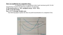
Business Economics, , s'o', , 6, , the Firm's, The Marginal Cost Curve and, The analysis of profit, a figure as given below:, , maximization can, , Supply, , I I (F.Y.B.Con.), , (Sem-, , Decision, , in the, be extended and explained, , form, , of, , MC, , MC, ATC, , P, , AV, , MC MC,, , MR, , =AR, , MC,, f, , QMAX, , Le, , Quantity, Fig. 1.1: Profit Maximization for a Competitive Firm, The marginal cost curve (MC) is upward sloping. The average total cost curve, (ATC) is 'U shaped. The MC curve crosses the ATC at the minimum of ATC (lowest, point). The figure shows a horizontal line at the market price (P). The price line is, , horizontal because the firm is a price taker. The price of the firm's output is the same, regardless of the quantity that the firm decides to produce. For a competitive firm the, , price, , AR = MR. The above figure can be used to find the quantity of output that|, , maximizes profit. Imagine that the firm is produced 0Q1. At this output level, MR is, greater than MC, which means that there is still scope to increase production and, earn more profit. At 0Q2 output level, MC> MR which means the firm should reduce, production. If the firm reduces production by 1 unit, the costs saved (MC) would, exceed the revenue lost (MR2). Thus when MR is less than MC, the firm can inerease, , profit by reducing production. The firm will eventually adjust production unti the, quantity produced reaches QMAX Thus, three general rules emerge from this with, , regard to profit maximization., 1., 2., , If MR is greater than MC, the firm should increase its output., , al, , If MC is, , cu, , greater than MR,, , the firm should decrease its, 3. At the profit maximizing level of output, MR = MC., , The above rules, , are, , the, , key, , to, , rational decision, , output., , making., , m, ex, , th-, , The, , following is an explanation of how, the competitive firm decides the, quantity o, its goods to be supplied to the market. Since, a, ATC, competitive firm is a price taker, 1s, AVCmarginal revenue equals the market price, For any given price, the, competitive firms, profit maximizing quantity of output, 18, found by looking at the, intersection of the, P%t, price with the marginal cost curve. In, figure above Fig. 1.1 that quantity of the, output, is, MAX Suppose the prevailing prices, the market rises due to increase in, Quantity, marke, demand. The figure, 1.2 shows how the, Fig., Fig. 1.2:Marginal Cost as the Competitive, competitive firm responds to the, firm's Supply Curve, price, MC, , P, , increase., , prma, ma, mE, , the, na, , tro, , COL, , tak, exE, , int, , det

Page 6 :
Market Structure : Perfect Competition and Monopoly, , 7, , g'g, , When the price is P1, the firm produces quantity Q1. This quantity Q, equates, MC to the price. When the price rises to P2, the firm finds that marginal revenue is, now higher than marginal cost at the previous level of output and so the firm, , increases production. The new profit maximizing quantity is Q2, at which marginal, , cost equals the new higher price. In short,since the firm's marginal cost curve, , determines the quantity of the good the firm is willing to supply at any price,, the marginal cost curve is also the competitive firm's supply curve. The firm, will not produce any output at a price below OPo, Since it will not be fully recovering, , its variable costs at a price below OP,. Thus, only the part of the short run, , marginal cost curve which lies above the AVC forms the short run supply, eurve of the firm., , Since under perfect competition, marginal cost curve must be, , rising above the minimum point of the AVC curve the short run supply curve of the, firm must always slope upwards to the right., , Long-run Market Supply, In the long run, firms will enter or exit the market until profit is driven to zero., As a result, price equals the minimum average total cost, as shown in panel (a). The, number of firms adjust to ensure that all demand is satisfied at this price. The long, run market supply curve is horizontal at this price, as shown in panel (b)., , MC, ATC, , Supply, , P=minimum ATCC, , Quantity, , Quantity (Market), , Fig. 1.3: (a) Firm's Zero Profit Condition, (b) Market Supply, , PERFECT COMPETITION, A perfectly competitive market achieves an efficient allocation of resources. The, , allocatively efficient output level occurs under perfect competition where the demand, curve intersects the supply curve. This is the point of equilibrium in a competitive, market. The perfectly competitive market model gives ideal' results which may not, exist in the real world. Perfect competition is defined as a market structure in which, there are a large number of price taking firms selling homogenous product., , The markets which display the features of perfect competition are those for, primary commodities. These are homogenous products which are sold in world, markets. Each individual supplier is small and hence cannot influence the world, , market. Each individual supplier is small and hence cannot influence the world, market price by actimg alone. Examples of perfectly competitive market conditions are, , the harket for cocoa beans, wheat, coffee beans, copper. Cocoa beans are the main, natural ingredient used in making chocolate. Cocoa beans grow on trees that require a, , tropical climate and substantial rainfall. There are eight major cocoa beans producing, countries and within these countries production is fragmented into a mixture of, , medium sized estates and small farms. In all ecases the farmers themselves are price, takers and are unable to influence the price that they receive. Thus, this market is an, example of perfect competition. The world market price is determined by the global, , interaction of demand and supply and each producer has to accept whatever price is, , determined.

Page 7 :
Business Economics, , g'R'S, , -, , l (F.YB.Com.) (Sem-, , features of perfert, and steel, the, copper, like, Even in the case of, is so large compared with, the world market, also, c, a, s, e, this, taker., competition c a n be seen. In, a, hence each firm is price, and, firms, the output of even the largest, competition may ba, structure. Perfect, market, of, one, type, Perfect competition is, number of firms producino, which there are large, in, situation,, defined as, 'that market, knowledge on the part, and free exit, perfect, free, entry, is, there, cost at all', homogeneous product,, aand no transportation, production, of, factors, of, mobility, of buyer, perfect, and produces an output, one among many, Under perfect competition, firm is, Hence it has no, of the total market supply., which forms a small or insignificant part, to adjust its, firm What it can do is, control over the market price. It is a price-taker, under traditional price, an assumption, output such that it makes maximum profit, , 8, , metals, , -, , theory., , decides to produce at a given, This profit maximisation output which a firm, is said to be in equilibrium, market price is the equilibrium output and the firm, minimum losses as in the short period)., making maximum profits or for that matter, , Features of Perfect Competition, Now let us discuss the features or conditions of perfect competition, i), , A large number of buyers and sellers, The number of sellers under perfect competition is assumed to be so large that the, share of each seller in the total supply of a product is very small. Any variation in the, output supplied by a single firm will not affect the total output of the industry. For the, , individual producers the price of the commodity is given. He can sell whatever output, he produces at the given price. Thus the firms are price takers and not price makers, The number of buyers are also so large that no single buyer or a group of buyers can, , influence the market price. As a result the demand curve under perfect competition is, infinitely elastic or is horizontal to the X-axis at the given price., , ii) Homogenous product, The commodities supplied by all the firms of an industry are homogeneous or, identical. Homogeneity of a product implies that one unit of the product is a perfect, substitute for another. Since the products are identical buyers are indifferent between, suppliers. Thus no firm can gain any competitive advantage over the other firms. The, homogeneity assumption rules out the possibility of charging different prices or higher, prices than prevailing in the market., , iii) Perfect mobility of factors of production, Another important characteristic of perfect competition is that the factors, of, production are freely mobile between the firms. For example, labour can freely move, from one firm to another or from one occupation to another as there are no barriers to, , mobility, legal, climate, skill, language, distance etc. In the same way capital, can also move freely from one firm to another. No firm has any kind of monopoly., As a, result, factors of production, land, labour, capital and entrepreneurship can enter or, quit a firm or the industry at will., iv) Free Entry and free exit, labour, , In a perfectly competitive market, there are no legal or market barriers on the, entry or exit of new firm to the industry or from industry. When the firms in the, , industry make supernormal profits new firms áre attracted to the industry. The entry, of new firms eliminate the super normal profits. When, profits decrease or more, , profitable opportunities are available elsewhere, firms leave the industry. The, , implication of this assumption 1s that given sufficient time, all firms in the industry, will be earning just normal profits.

Page 8 :
9, , Market Structure: Perfect Competition and Monopoly, , )Porteet knowledge, The, sellers have perfect. knowledgo about the markot conditions., the prevailing and future prices, buyers and sellers have full information regarding, and insecurity, and availability of the commodity. In such a situation, uncertainty, about the future developments in the market is ruled out., , Thebuyers and, , vi) No (Government interforence, There a r e no, Government does not interfere in the functioning of the market., of inputs by the, discriminatory taxes or subsidies no licensing system, no allocation, Thus the government, government or any other kind of direct or indirect control., , follows the free enterprise policy., , vii) Absence of collusion and independent decision making by firms, a r e not in, It is assumed that there is no collusion between the firms and they, are also not in any, league with one another in the form of guild or cartel. The buyers, etc. The firms and, kind of collusion among themselves like consumer's association, , buyers take their decisions independently and they act independently., -, , REVENUE CONCEPTS, Total Revenue, Average Revenue and Marginal Revenue, , Since the decision of a firm in respect of what output it should produce depends, We, to study how a firm calculates its profits., upon the level of profit, it is necessary, of a firm, its average, shall, therefore, introduce three concepts viz. total r e v e n u e, revenue and its marginal revenue., firm from, Total Revenue. Total Revenue is the sum total of receipts earned by a, measured by price per unit, selling its outputs. The total r e v e n u e at any output is, r e v e n u e is a function of, multiplied by quantity sold (price x total output sold). Total follows:, as, sales which a r e equal to output. This function maybe written, , Px=f, ), where P stands for price and, , x, , denotes output., , Px, therefore,, , denotes total, , revenue., , Average Revenue, Average Revenue m e a n s revenue per unit, price. Average revenue is calculated as under, Average revenue, If the total, average, , Total revenue or AR =, , revenue, , revenue, , 400, is 100, , Total output, , of output. This is the, , same, , thing, , as, , where r stands for total output., , is { 400/- and the total output sold is 100 units, , only,, , then the, , 4., , Marginal Revenue, is the addition to the total revenue by the sale of a n, additional unit of output., and the second at 95 paise, the, Suppose the first unit is sold at 100 paise, units of output is 95 paise. The total revenue, marginal r e v e n u e in respect of the two, first unit is, from the two units is 195 paise. Since the total r e v e n u e from the, , Marginal, , revenue, , 100 paise, the marginal revenue, or the revenue added by the sale of the second unit,, units of a, is 95 paise. If we want to know the marginal revenue of 'n' (any nunmber), and subtract from it the, good, we should, first calculate the total revenue from n units, , totalrevenue fromn-1 units., Thus, MR of n units can be mathematically, , MR, TR-TRn-1, , written, , as, , under:

Page 9 :
Business Economics l l (F.Y.B.Com.) (Sem-, , 10, , ), , MR can also be written in a derivative form., , MR=K, d, , (incremental TR due to, , a, , unit change in output)., , where TR stands for Total Revenue, and 'n' for any given number of units., Y, , (B), , (A), S, , Q, -PE, , -X, -, , QUANTITY., , Fig. 1.4 A &B, , TheEquilibrium Price, , The equilibrium price is decided by the industry supply and demand curves, , Fig. 1.4 (A). An individual firm is a price-taker. The PQ curve in Fig. 1.4 (B) is both, the average revenue curve and the marginal revenue curve., , 6, , IMPORTANT OBSERVATION, Since we are assuming the existence of perfect competition, the marginal|, , revenue and average revenue would be equal1., This is because a firm is a price-taker and can produce any quantity of output at, , the prevailing equilibrium price. This equilibrium price is the result of demand and, supply prevailing in the market (See Fig. 1.4 A and B)., , The equilibrium price in the market is OP, which is decided by demand-and, supply forçes. Since the firm is a price-taker, OP will be its prices and it can produce, any output and sell it at that price. Since every additional unit is sold at the same, price, the revenue added (i.e. marginal revenue) equals the price or average revenue., For a firm, therefore, average revenue and marginal revenue would be equal under, conditions of perfect competition. See the following revenue schedule:, , Table:1.2:Revenue Schedule of AFirm, Price, , ), , Units of, , Total, , Average, , Marginal, , sugar sold, , Revenue, , Revenue, , Revenue, , (TR), 100, , 500, , 5, , 5, , 5, , 101, , 505, , 5, , 5, , 5, , 102, , 510, , 5, , 5, , 5, , 103, , 515

Page 10 :
Market Structure: Perfect Competition and Monopoly, , 9'o'R, , Profits Defined, , 11, , firm's total profits are equal to the, difference between its total, total costs, Total profits Total revenue Total costs., A, , revenue and, , =, , -, , We, a, , TC, TR, , B, P, D, , show the maximum, , can, , firm with, , a, , profit output., , of, , diagram (See Fig 1.5)., , The verticle distance PQ, represents, total profit which is the maximum., In Fig. 1.5, TC is the total cost curve and TR, the total revenue curve. The firm will make the, maximum profit when the vertical distance, between the TR and TC curves is the biggest, , possible. This distance is PQ. At output OM, the, , slopes of TC and TR curves are equal. PQ is the, , distance where tangents AB and CD to the TR, , Q, , and TC, , curves, , respectively are parallel., , This can be shown by using calculus as, , M, , OUTPUT, , under, , Fig. 1.5: Maximum Profit Output, The total revenue is a function of output., The total revenue is equal to price multiplied by the output sold. Then we can show, this function by the following equation:, Px =, , f), , (Px denotes total revenue, i.e., Price P multiplied by output x)., The total cost is, , a, , function of output., , Thus, C = F (x), , C denotes total cost which is a function of total output a)., To get the maximum difference between the two functions, we should find that, , value of r (output) where the derivatives of the two functions are equal. Thus,, , PxdC, dx, In Fig. 1.5, this equality of the derivatives of the two functions occurs where x is, , equal of OM. The tangent AB represents the derivative of the total revenue function, and tangent CD represents the derivative of the total cost function. We may say that, , profits are maximum when the derivatives of the total cost function and the total, revenue function are equal., , Firm's Equilibrium Output under Perfect Competition; conditions for, , equilibrium, An equilibrium is a situation in which economic forces have no tendency to, , change., A firm is said to be in equilibrium when an entrepreneur has no motive to change, , his organisation or the scale of his operations. In such circumstances, he will not wish, change the proportion in which the factors of production are combined or to change, output, as either will result in a smaller profit., to, , We would say that such an equilibrium of a firm will occur when it, , makes maximum profit; for it is only then that the entrepreneur will have no, desire to change the level of output by adding or reducing factors of, , production.

Page 11 :
Business Economics, 12, level, , of output, , is, , -, , |l, , (F.Y.B.Com.) (Sen, , OM because, at th, , In Fig. 1.5, we can see, If the output 18 reduced h., profit., maximum, total revenue and, level of utput, the firm makes the, between the, distance, vertical, totalorcostcreased, curves will, be less, the PQ. In other words, the total profit will, ibrium, be le8s, level, OM,than, beyond, OM, that the, , the maximum. We,, output for the firm., , quilibrium, , detailed i n t o r m a t i o n as, , any, we do not get, However, in this kind of figure,, marginal, average revenue,, price. We, therefore, use the, , marginal cost concepts., , While, , than, , is the equilibr, this OM output, that, therefore, say, , analysing the, , condition for, , a, , revenue,, , firm's equilibrium,, , we, , rea, , egards, , average cost, , shall, , consider, , and, two, , periods separately, 1., , the short period and, , 2. the long period., , Short Period and Firm's Equilibrium, , help of variahl., its output only with, 1able, a firm can increase, In, short, period,, factors. the, Some, factors, like machinery, plant, etc., are fixed. It would take a long period, the, , to instal new plant or to fix new machinery. Therefore, it is not possible for new firma, to enter an industry in the short period., , Conditions of Short-Period Equilibrium, The short-period equilibrium position is, , MC, , that of maximum profits (or minimum losses), for a firm. The firm's equilibrium output is, that output where two conditions are, , 8., , AR=MR, , satisfied, 1. The marginal cost is equal to the, , Equilibrium point, , marginal revenue. MR = MC., , 2. The marginal cost curve should cut, , the marginal revenue curves from, below (See Fig. 1.6)), The firm's equilibriúm position is at, , N, , OUTPUT, , Fig. 1.6:Short Period Equilibrium of, Firm, , point R., At, , M, , point R, both, , the, , conditions, , satisfied MR = MC and MC, curve from below. The equilibrium output is OM when the price is OP., are, , curve, , cuts M, , Why MR and MC should be Equal at an Equilibrium Point, We have seen in Fig. 1.5 that a firm's profits are maximum, at that level of output, where the vertical distance between total cost and total, revenue is as great, possible. At this output, the slopes of tangents to the total cost curve and total revenue, curve are equal, since these tangents are, parallel., Now the tangent to the total, revenue curve represents a derivative of the, tour, revenue function, while the tangent to the total cost, curve represents a derivative, the total cost function. Thus, maximum profits occur, when these two derivatives, equal., , dP)_dC, where P is, Since, , price, x, , marginal, , 18 total, , revenue, , of, , is, , output, a, , the total, c0st is a derivative, maximum profits when MR = MC., , dx, , and C is total, cost., , erivative, , of the total, cost function, we revenue function and margn, may say that a firm will ear, , f, sL, , a, , a, , Va, to, Si, , Al, fa

Page 12 :
-ID, , his, ow, , che, an, of, , rds, nd, wo, , 13, , g'o'R, , Market Structure Perfect Competition and Monopoly, , Why MC should cut MR Curve from Below, R, While referring to Fig. 1.6 we find that MC and MR are equal at points Q and, even, (at two levels of output ON and OM). But point Q cannot be an equilibrium point, though MC and MR are equal at that point because, at this point, profits are, minimum. They are minimum because the firm has further scope to expand output, which, beyond ON and earn extra revenue which is shown by the shaded area and, the excess of additional revenue over additional cost. Profits will inerease,, , represents, , if the output is extended to OM quantity., Thus, it is only at R that the firm makes maximum profits. The second condition, therefore, ightly states that the MC curve should cut the MR curve from below. R is, , the point of maximum profit and Q is the point of minimum profit., Profits and Super-normal Profits, Normal, Normal Profits : The total cost includes the minimum profits which a, , producer, , expects to get in order to remain in the industry. These are known as "Normal, , ble, iod, ms, , Profits". Normal profits may be defined as that amount of money which is just, , sufficient to induce the firm to stay or continue in the industry., , This amount of normal profits is included in the total cost of production. The, average cost curve shows both-the actual cost per unit plus the amount of normal, profits per unit. When the average cost is recovered, it means that the firm is making, normal profits. This situation exists when the price or average revenue is equal to the, average cost. See Fig. 1.7 (B). There are only normal profits at point 'D', , Super-normal Profits: If the price (AR) is greater-than the average cost, the, firm makes more than normal profits. These profits are known as "Super-normal", profits or abnormal profits. Every firm will be happy when it gets normal profit, but it, is happier when the price (AR) is so high (higher than the average cost) that it enjoys, super-normal profits., , Numerical Example, , MR, , For example, if the actual total cost of production is 1000 at the output level of, 100 units, and the market rate of interest is 15 per cent, then the producer will expect, at least 7 150 as minimum profit on his investment ofT 1000. This is because had he, lent the said amount, he could have earned 150 by way of interest since the market, rate of interest is 15 percent. This amount is the normal profit which the firm must, get in order to stay in the industry. Otherwise it is better to lend money at 15 per cent, and receive 7 150 instead of investing it in production., In our above example the total cost will be F 1,150, , put, as, , ue, tal, , of, , are, , 100 units. The average cost is, , 1,000 plus 7 150) for, , 11.50. If the price (AR) in the market is 7 11.50, the, , firm makes normal profits. If the price is higher, say, , 14, then the firm makes the, , super-normal profit ofR 2.50 per unit sold. Note that super-normal profits are in, addition to the normal profits. In the diagram, the supernormal profits aremeasured, by the vertical distance between the AR curve and the average cost curve. In, Fig. 1.7 A, area CB shows average supernormal profits. The total supernormal profits, are shown by the shaded area APCB., , Various Equilibrium Situations, Now we can refer to the other costs of a firm in the short, period. viz., aver?ge, total units cost and average variable cost and find out the, various equilibrium, , situations for a firm at various given prices., , nal, arn, , All Factors are Homogeneous, We, , assume, , that all factors of, , production, , homogeneous., factor prices for all firms; and so all firms have identical, costs curves., are, , There, , are, , identical

Page 13 :
Business Economics-II(F.Y.B.Com), 14, Firm's Equilibirum-Short Period, , (AII, , Factors, , (Sem,, , Homogeneous), , is-somcthin, , additional anmount (that, some, expect, firm, may, the, that, because of extra cftorts or, lt 1s possible, or normal profit, minimum, the, more than 15 per cent) as, troubles involved in production business., D is called break-even, in ATUC. Point, are included, which, Only normal profits, 1.7 (B)), 'D' and output is OM,. (Fig., point. The equilibrium point is, the product. Equilibrium, to lower price for, due, losses, shows, ABE, area, Shaded, P2, minimum losses., but the firm is making, and, 'E', OM9,, is, output, point, Break Evcn Point, , MC, Super Normal, , ATUC, , AVC, , ATUC, , ML, , Normal Profits, , AVC, , Profits, , AR-MR, =MR, , MR =MC, AR>ATUC, MR=MC, , AR-ATUC, , X, , M, , M, , OUTPUT, , OUTPUT, , Fig., , Fig. 1.7 (A) : Super Normal Profits, , 1.7, , (B), , :, , Normal Profits, , cost of, normal profit maybe estimated on the basis of the opportunity, in the next best, the entrepreneur's labour-that is equal to what he could have earned, Minimum, , or, , alternative job., Explanation of figures 1.7 A, B and C, , sE, , Fig. 1.7 (A) : In this figure, the point of, , equilibrium is C where MR and MC are equal., MC, , The equilibrium output for each firm is OM. If, we draw a perpendicular CM from point C, towards the X-axis, we can read on it the, , AR-MR, , 9, , Since the average revenue is greater than the, average cost, the firm makes more than normal, profits or supernormal profits., , MR-MC, , ATUC> AR, , The total profits are shown by the shaded, area APCB, which are the maximum profits., , The total revenue is equal to the area OPCM, and the total cost is equal to the area OABM, , AVC, , Losses, , average revenue CM at OM output, average P 2, fixed cost BF and average variable cost FM., , ATUC, , X, , M2, OUTPUT, , Fig. 1.7 (C) : Short Period Losses, , The difference between the two (OPCM-0ABM) is total profit. If the price of the, product' increases, the firm's supernormal profits will be still higher., Fig. 1.7 B :In Fig. 1.7 B, the price has decreased and the equilibrium point for, each firm is D, where MC and MR are equal. Here, the equilibrium output is OM, , Average revenue is DM1 and average cost is also DM1; both are equal. A firm makes, , At, , only normal profits (which are included in the average total unit cost). This point, , pa, , maybe called the, k-even point, because all costs (fixed and variable) have bee, een, recovered by the firm. At this point, the marginal revenue curve is tangent to tn, , fir, , ATUC curve. This is a point of minimum average total unit cost.

Page 14 :
Market Structure: Perfect Competition and Monopoly, , 15, , Fig. 1.7 C :ln this figure, the price hns dropped further and the new equilibrium, point for each firm is E and the equilibrium output in OM, If we look at the, , perpendicular drawn from point E to X-axis, we find that AR is EM, , and is less than, , the average total unit cost BM2. Since AR is less than ATUC, the firm is incurring, losses, which are the minimum losses. The variable cost (FM) is completely recovered, , and only some part of the fixed cost is recovered. In Fig. 1.7 C, each firm incurs a total, loss equal to P2ABE (shaded area). Total revenue is OPEM2 and total costs are, , OABM., If the price falls further, the losses of each firm will increase. In the short period,, a firm has already incurred its fixed costs. If it closes down, it will be losing all its, fixed costs. It will, therefore, be in the interest of the firm to stay in business and, recover as much of its fixed costs as possible and avoid a total loss of these costs. We, , may, therefore, conclude that a firm will continue to produce despite the losses it has, incurred. So long as it can recover its variable costs and recover some amount of fixed, costs, a firm will continue in the industry., , Shut-Down Point, If the price drops further and the firm cannot even recover its variable costs, it, will be in its interest to close down and avoid losses in terms of variable costs, , (See Fig. 1.8 A.)., We may say that a firm will continue in the industry so long as, at least, it, recovers its fill variable costs. In other words, the average revenue should at least be, , equal to the average variable cost. This point is S in Fig. 1.8 B. This point is called the, shut-down point., Shut-down point or last price = AVC, , OP is the last price at which a firm will continue to operate in the industry in the, short period. It is equal to AVC. If the price falls below AVC, it will close down., Y, , (B), , (A), ATUC, , MC, , MC, , ATUC, , AVC, , AVC, , N, , P, , AR=MR, , AR-MR, , hut down Point, MR-MC, , Firm will close down, , (AR<AVC), , AR-AVC, , X, , M, , N, , OUTPUT-, , Fig. 1.8 (A), Close Down Point, , At OPj price, the firm loses even some, , part of the variable cost (N No). The, firm will close down., , Fig. 1.8 (B), Shut Down Point, , At OP price, the firm is in equilibrium at, point S. It just recovers its variable cost, SM. This point is called the shutdown, , point. If the price falls below OP, the, firm will shut-down.

Page 15 :
Com.)(Sem, , Business Economics- ll (E.Y.B.Com.) (Sem, , 16, The, , following table gives, , us an, , normal profit, supernormal proits,, idea about, , and, , losses., , Table. 1,3, Relation between AR, , ,, , (Priceand AC), Supernormalprofits., , AR>AC, , 1., , AR, , Normal profit-break-even point., , AC, , 3., , AR < AC, , 4., , AR AVC, , Losses., Shut-down point. This is the last price, , A firm will close down., , AR< AVCc, , 5., , at, , which a firm will operate., , Entrepreneurs Heterogeneous and Other Factors, , Homogeneous, Now we can drop the assumption that all factors are homogeneous. First, we, , consider the situation where producers are of diferent efficieney (heterogeneous) and, other factors are homogeneous. More efficient producers will produce more efficientiy,, their costs will be lower. Less efficient producers will produce less efficiently : they, will incur higher costs., , MC, , 0, , M, , MC, , MC, , ATUd, Avd, P ZIEHLI F, , D, , C, , B, , A, , MC ATUC, , ATUC, , ATUC, , AVC, , AVC, , th, , AVC, , --, , SDAR-MR, , o, , M, , X, , W, , X, , X, , O, , St, , OUTPUT, , ec, , Fig. 1.9:(A), (B), (C), (D), Heterogeneous Entrepreneurs, , (A), , (B), , Firm which more, efficient make, supernormal, , profits (shown by, , or, , th, , (C), , D), , Less efficient, , Less efficient, , producers makes, only normal profits, , A very inefficient, , producer makes a, loss (shown by, shaded area)., , producer cannot, even recover his, variable costs, He, , (AR, , ATUC)., , shaded area)., , has to close down., , The maximum profits of the more efficient, producers will be greater than those, the less efficient producers. Less effñcient firms, may incur losses. Some firms, may, so inefficient that they may not, to, recover, be able, their high variable costs. Such, fir, will close down. See Fig. 1.9 A-B-C-D., , All Factors Heterogeneous, When all factors of production are, heterogeneous, those employing more enticient, factors will greatly reduce their costs and the, firms employing lessefficient tactors (inefficient, producer,in low, labour, theand, costso, difference, theirquality, costs and, , materials, etc.), , will be greaer, , than that as, , ra, , shown in., , Fig., , 1.9, , A, B, C and D., , ot, to, in, , ob, an, , po, , eq, CoE, , eq, , fac

Page 16 :
Market Stucture: Pefect Competition and Monopoly, A firm with, , 'o', more efficient producers employing more efficient labour,, , 17, , will reduce, , its average total unit cost substantially and will, therefore, earn even more profit than, that shown in Fig. 1.9 (A)., , Firms making losses will make more losses than that shown in Fig. 1.9 (C). Firms, , employing very poor factors will have to close down, if they are unable to recover even, their variable costs., I, , firm, , ONG PIRtOD, , EQULRUM (INDUSTRY EQUILIBRIUM), , A long period is defined as the period when all factors of a firm are variable. A, can change its plant; it, may double its size or reduce it to half. New firms may, , enter an industry, if the existing firms are earning supernormal profits; or some, , existing firms may close down permanently, if they continue to incur losses and have, no capacity to bear such losses., , Conditious, A long-period equilibrium will be that situation in which the following two, conditions are fulfilled, , a) Each firm in the industry is in equilibrium., b) The whole industry is also in equilibrium., This means that there should be no attraction for, and no worry for the existing firms to close down., , new, , firms to enter the, , industry, , The first condition is required to ensure that each firm makes the maximum, profits. This condition is fulfilled when MR and MC are equal and the MC curve cuts, the MR curve from below :, The second condition is required to ensure that there is no entry of new firms into, the industry or that no existing firms leave it. This will happen when there are, , neither supernormal profits, nor are there any losses., When are new firms attracted towards an industry? It is when there are, , supernormal profits. When will an existing firm be anxious to close down? Obviously,, when it incurs losses in terms of its fixed costs., , Y, , So the second condition of a long-period, equilibrium is fulfilled when all firms make, , MC, , AC, , only normal profits. This is the position when, , the, , total revenue is equal to the total cost. In, other words, average revenue should be equal, to the average cost. Thus, a long-period, , AR=MR, , industry equilibrium is established when we, obtain two conditions, viz., A. MR = MC, MC cutting MR from below;, and, , of, be, , ns, , nt|, , of, aw, , M, OUTPUT, , X, , Fig. 1.10 : Long - Period Equilibrium, , B. AR = AC (MR = MC =AR = AC)., , This is the minimum point on the average cost curve and MC passes through this, point. The AR curve is tangent to AC at this point. In other words, a firm's, , equilibrium level of output will be that where, marginal revenue is equal to marginal, cost, is equal to average revenue, is equal to average cost (See Fig. 1.10)., MR =MC = AR = AC, The equilibrium point is Q where MR = MC and at the same point AR = AC. The, , equilibrium output of each firm is OM. There are only normal profits., Assuming that in all the firms in an industry, homogeneous (equally efficient), factors are employed, each firm in the industry will have identical costs and, produce

Page 17 :
Business, , at the minimum average, , cost., , n the, , and, , we, , call, , whole industry, noted, the, be, should, short period, it, , Supernormal profits, , or, , Sem-, , S, , output. ."The, , produce, will also e q u i l i b r i u m ., Each firm, this full, , is in uilibriur, industry, equilibrium., Why? Even though, , whole, , (F.YB.Com.), , the optim, imum, , g's's, , 18, , EconomicslI, , may not, , be in f, , each firm is in equilibrium, all firms may bebemsaid to, , the, and hence, incurring losses, , cannot, whole i n d u s t r y, , be s o, , Long period equilibrium, , be in equilibrium., MC, , MC, , B, , th, , AC, , S, , AC, , 3, , SL, , AR, , AR MR, , MR, , no, , X, , pe-, , M, , X, AC, , MC, , D, , ex, , AC, , kn, , MC, , C, , des, AR= MR, , Me, R, , MR, , po, car, , M, , var, , M, , OUTPUT-, , fall, , Fig. 1.11: (A), (B), (C), (D), Process of Long Period Equilibrium, , Firms are earning, Bupernormal, profits. New firms, will start entering, , the industry in the, long period., , The price will fall | Firms incur losses, , to, , OP1, , and, , area)., , all | (shaded, , will, normal leave the industry, earn Some, , firms, , will, , only, profits., , The whole, , industry, equilibrium., , 1s, , in, , the, , firms, , long period., , in, , Firms, , profits., (B), , LRMC, , will, , normal, , earn, , LRMC, , has, , When some firms, the., leave, Industry,, industry's supply, will decrease and, price will rise to, , OP1, , (A), , (se, , D, , C, , B, , A, , LRAC, , sel, mol, , clos, anc, , ind, , elas, zerc, , LRAC, AR = MR, , Sup, , eve, ther, cou, mor, M, , x, OUTPUT, , Mi, , Fig. 1.12 (A), , Most efficient Firm (Long Period), , Fig. 1.12 (B), , Marginal Firm (Long Period), , Tele