Page 1 :
the essentials of, , Linda Null and Julia Lobur, , JONES AND BARTLETT COMPUTER SCIENCE
Page 2 :
the essentials of, , Linda Null, Pennsylvania State University, , Julia Lobur, Pennsylvania State University
Page 3 : World Headquarters, Jones and Bartlett Publishers, 40 Tall Pine Drive, Sudbury, MA 01776, 978-443-5000,
[email protected], www.jbpub.com, , Jones and Bartlett Publishers, Canada, 2406 Nikanna Road, Mississauga, ON L5C 2W6, CANADA, , Jones and Bartlett Publishers International, Barb House, Barb Mews, London W6 7PA, UK, , Copyright © 2003 by Jones and Bartlett Publishers, Inc., Cover image © David Buffington / Getty Images, Illustrations based upon and drawn from art provided by Julia Lobur, Library of Congress Cataloging-in-Publication Data, Null, Linda., The essentials of computer organization and architecture / Linda Null, Julia Lobur., p. cm., ISBN 0-7637-0444-X, 1. Computer organization. 2. Computer architecture. I. Lobur, Julia. II. Title., QA76.9.C643 N85 2003, 004.2’2—dc21, 2002040576, All rights reserved. No part of the material protected by this copyright notice may be reproduced or utilized in, any form, electronic or mechanical, including photocopying, recording, or any information storage or retrieval, system, without written permission from the copyright owner., Chief Executive Officer: Clayton Jones, Chief Operating Officer: Don W. Jones, Jr., Executive V.P. and Publisher: Robert W. Holland, Jr., V.P., Design and Production: Anne Spencer, V.P., Manufacturing and Inventory Control: Therese Bräuer, Director, Sales and Marketing: William Kane, Editor-in-Chief, College: J. Michael Stranz, Production Manager: Amy Rose, Senior Marketing Manager: Nathan Schultz, Associate Production Editor: Karen C. Ferreira, Associate Editor: Theresa DiDonato, Production Assistant: Jenny McIsaac, Cover Design: Kristin E. Ohlin, Composition: Northeast Compositors, Text Design: Anne Flanagan, Printing and Binding: Courier Westford, Cover Printing: Jaguar Advanced Graphics, This book was typeset in Quark 4.1 on a Macintosh G4. The font families used were Times, Mixage, and Prestige, Elite. The first printing was printed on 45# Highland Plus., Printed in the United States of America, 07 06 05 04 03, , 10 9 8 7 6 5 4 3 2 1
Page 4 :
In memory of my father, Merrill Cornell, a pilot and man of endless talent and courage,, who taught me that when we step into the unknown, we either find solid ground, or we, learn to fly., —L. M. N., To the loving memory of my mother, Anna J. Surowski, who made all things possible for, her girls., —J. M. L.
Page 6 :
PREFACE, , TO THE STUDENT, his is a book about computer organization and architecture. It focuses on the, , Tfunction and design of the various components necessary to process informa-, , tion digitally. We present computing systems as a series of layers, starting with, low-level hardware and progressing to higher-level software, including assemblers and operating systems. These levels constitute a hierarchy of virtual, machines. The study of computer organization focuses on this hierarchy and the, issues involved with how we partition the levels and how each level is implemented. The study of computer architecture focuses on the interface between, hardware and software, and emphasizes the structure and behavior of the system., The majority of information contained in this textbook is devoted to computer, hardware, and computer organization and architecture, and their relationship to, software performance., Students invariably ask, “Why, if I am a computer science major, must I learn, about computer hardware? Isn’t that for computer engineers? Why do I care, what the inside of a computer looks like?” As computer users, we probably do, not have to worry about this any more than we need to know what our car looks, like under the hood in order to drive it. We can certainly write high-level language programs without understanding how these programs execute; we can use, various application packages without understanding how they really work. But, what happens when the program we have written needs to be faster and more, , v
Page 7 :
vi, , Preface, , efficient, or the application we are using doesn’t do precisely what we want? As, computer scientists, we need a basic understanding of the computer system itself, in order to rectify these problems., There is a fundamental relationship between the computer hardware and the, many aspects of programming and software components in computer systems. In, order to write good software, it is very important to understand the computer system as a whole. Understanding hardware can help you explain the mysterious, errors that sometimes creep into your programs, such as the infamous segmentation fault or bus error. The level of knowledge about computer organization and, computer architecture that a high-level programmer must have depends on the, task the high-level programmer is attempting to complete., For example, to write compilers, you must understand the particular hardware, to which you are compiling. Some of the ideas used in hardware (such as pipelining) can be adapted to compilation techniques, thus making the compiler faster, and more efficient. To model large, complex, real-world systems, you must, understand how floating-point arithmetic should, and does, work (which are not, necessarily the same thing). To write device drivers for video, disks, or other I/O, devices, you need a good understanding of I/O interfacing and computer architecture in general. If you want to work on embedded systems, which are usually very, resource-constrained, you must understand all of the time, space, and price tradeoffs. To do research on, and make recommendations for, hardware systems, networks, or specific algorithms, you must acquire an understanding of, benchmarking and then learn how to present performance results adequately., Before buying hardware, you need to understand benchmarking and all of the, ways in which others can manipulate the performance results to “prove” that one, system is better than another. Regardless of our particular area of expertise, as, computer scientists, it is imperative that we understand how hardware interacts, with software., You may also be wondering why a book with the word essentials in its title is, so large. The reason is twofold. First, the subject of computer organization is, expansive and it grows by the day. Second, there is little agreement as to which, topics from within this burgeoning sea of information are truly essential and, which are just helpful to know. In writing this book, one goal was to provide a, concise text compliant with the computer architecture curriculum guidelines, jointly published by the Association for Computing Machinery (ACM) and the, Institute of Electrical and Electronic Engineers (IEEE). These guidelines encompass the subject matter that experts agree constitutes the “essential” core body of, knowledge relevant to the subject of computer organization and architecture., We have augmented the ACM/IEEE recommendations with subject matter, that we feel is useful—if not essential—to your continuing computer science, studies and to your professional advancement. The topics we feel will help you in, your continuing computer science studies include operating systems, compilers,, database management, and data communications. Other subjects are included, because they will help you understand how actual systems work in real life.
Page 8 :
Preface, , vii, , We hope that you find reading this book an enjoyable experience, and that, you take time to delve deeper into some of the material that we have presented. It, is our intention that this book will serve as a useful reference long after your formal course is complete. Although we give you a substantial amount of information, it is only a foundation upon which you can build throughout the remainder, of your studies and your career. Successful computer professionals continually, add to their knowledge about how computers work. Welcome to the start of your, journey., , TO THE INSTRUCTOR, About the Book, This book is the outgrowth of two computer science organization and architecture, classes taught at The Pennsylvania State University Harrisburg campus. As the, computer science curriculum evolved, we found it necessary not only to modify, the material taught in the courses but also to condense the courses from a twosemester sequence into a three credit, one-semester course. Many other schools, have also recognized the need to compress material in order to make room for, emerging topics. This new course, as well as this textbook, is primarily for computer science majors, and is intended to address the topics in computer organization and architecture with which computer science majors must be familiar. This, book not only integrates the underlying principles in these areas, but it also introduces and motivates the topics, providing the breadth necessary for majors, while, providing the depth necessary for continuing studies in computer science., Our primary objective in writing this book is to change the way computer, organization and architecture are typically taught. A computer science major, should leave a computer organization and architecture class with not only an, understanding of the important general concepts on which the digital computer is, founded, but also with a comprehension of how those concepts apply to the real, world. These concepts should transcend vendor-specific terminology and design;, in fact, students should be able to take concepts given in the specific and translate, to the generic and vice versa. In addition, students must develop a firm foundation for further study in the major., The title of our book, The Essentials of Computer Organization and Architecture, is intended to convey that the topics presented in the text are those for which, every computer science major should have exposure, familiarity, or mastery. We do, not expect students using our textbook to have complete mastery of all topics presented. It is our firm belief, however, that there are certain topics that must be mastered; there are those topics for which students must have a definite familiarity; and, there are certain topics for which a brief introduction and exposure are adequate., We do not feel that concepts presented in sufficient depth can be learned by, studying general principles in isolation. We therefore present the topics as an inte-
Page 9 :
viii, , Preface, , grated set of solutions, not simply a collection of individual pieces of information. We feel our explanations, examples, exercises, tutorials, and simulators all, combine to provide the student with a total learning experience that exposes the, inner workings of a modern digital computer at the appropriate level., We have written this textbook in an informal style, omitting unnecessary jargon, writing clearly and concisely, and avoiding unnecessary abstraction, in, hopes of increasing student enthusiasm. We have also broadened the range of topics typically found in a first-level architecture book to include system software, a, brief tour of operating systems, performance issues, alternative architectures, and, a concise introduction to networking, as these topics are intimately related to, computer hardware. Like most books, we have chosen an architectural model, but, it is one that we have designed with simplicity in mind., Relationship to Computing Curricula 2001, In December of 2001, the ACM/IEEE Joint Task Force unveiled the 2001 Computing Curricula (CC-2001). These new guidelines represent the first major revision since the very popular Computing Curricula 1991. CC-2001 represents, several major changes from CC-1991, but we are mainly concerned with those, that address computer organization and computer architecture. CC-1991 suggested approximately 59 lecture hours for architecture (defined as both organization and architecture and labeled AR), including the following topics: digital, logic, digital systems, machine-level representation of data, assembly-level, machine organization, memory system organization and architecture, interfacing, and communication, and alternative architectures. The latest release of CC-2001, (available at www.computer.org/education/cc2001/) reduces architecture coverage to 36 core hours, including digital logic and digital systems (3 hours),, machine-level representation of data (3 hours), assembly-level machine organization (9 hours), memory system organization and architecture (5 hours), interfacing and communication (3 hours), functional organization (7 hours), and, multiprocessing and alternative architectures (3 hours). In addition, CC-2001 suggests including performance enhancements and architectures for networks and, distributed systems as part of the architecture and organization module for CC2001. We are pleased, after completely revising our course and writing this textbook, that our new material is in direct correlation with the ACM/IEEE 2001, Curriculum guidelines for computer organization and architecture as follows:, AR1., AR2., AR3., AR4., AR5., AR6., AR7., , Digital logic and digital systems (core): Chapters 1 and 3, Machine-level representation of data (core): Chapter 2, Assembly-level machine organization (core): Chapters 4, 5 and 6, Memory system organization and architecture (core): Chapter 6, Interfacing and communication (core): Chapter 7, Functional organization (core): Chapters 4 and 5, Multiprocessing and alternative architectures (core): Chapter 9
Page 10 :
Preface, , ix, , AR8. Performance enhancements (elective): Chapters 9 and 10, AR9. Architecture for networks and distributed systems (elective):, Chapter 11, Why another text?, No one can deny there is a plethora of textbooks for teaching computer organization and architecture already on the market. In our 25-plus years of teaching these, courses, we have used many very good textbooks. However, each time we have, taught the course, the content has evolved, and, eventually, we discovered we, were writing significantly more course notes to bridge the gap between the material in the textbook and the material we deemed necessary to present in our, classes. We found that our course material was migrating from a computer engineering approach to organization and architecture toward a computer science, approach to these topics. When the decision was made to fold the organization, class and the architecture class into one course, we simply could not find a textbook that covered the material we felt was necessary for our majors, written from, a computer science point of view, written without machine-specific terminology,, and designed to motivate the topics before covering them., In this textbook, we hope to convey the spirit of design used in the development of modern computing systems and what impact this has on computer science students. Students, however, must have a strong understanding of the basic, concepts before they can understand and appreciate the non-tangible aspects of, design. Most organization and architecture textbooks present a similar subset of, technical information regarding these basics. We, however, pay particular attention to the level at which the information should be covered, and to presenting, that information in the context that has relevance for computer science students., For example, throughout this book, when concrete examples are necessary, we, offer examples for personal computers, enterprise systems, and mainframes, as, these are the types of systems most likely to be encountered. We avoid the “PC, bias” prevalent in similar books in the hope that students will gain an appreciation for the differences, similarities, and the roles various platforms play within, today’s automated infrastructures. Too often, textbooks forget that motivation is,, perhaps, the single most important key in learning. To that end, we include many, real-world examples, while attempting to maintain a balance between theory and, application., Features, We have included many features in this textbook to emphasize the various concepts in computer organization and architecture, and to make the material more, accessible to students. Some of the features are listed below:, • Sidebars. These sidebars include interesting tidbits of information that go a, step beyond the main focus of the chapter, thus allowing readers to delve further into the material.
Page 11 :
x, , Preface, , • Real-World Examples. We have integrated the textbook with examples from, real life to give students a better understanding of how technology and techniques are combined for practical purposes., • Chapter Summaries. These sections provide brief yet concise summaries of, the main points in each chapter., • Further Reading. These sections list additional sources for those readers who, wish to investigate any of the topics in more detail, and contain references to, definitive papers and books related to the chapter topics., • Review Questions. Each chapter contains a set of review questions designed to, ensure that the reader has a firm grasp on the material., • Chapter Exercises. Each chapter has a broad selection of exercises to reinforce the ideas presented. More challenging exercises are marked with an, asterisk., • Answers to Selected Exercises. To ensure students are on the right track, we, provide answers to representative questions from each chapter. Questions with, answers in the back of the text are marked with a blue diamond., • Special “Focus On” Sections. These sections provide additional information, for instructors who may wish to cover certain concepts, such as Kmaps and, input/output, in more detail. Additional exercises are provided for these sections as well., • Appendix. The appendix provides a brief introduction or review of data structures, including topics such as stacks, linked lists, and trees., • Glossary. An extensive glossary includes brief definitions of all key terms, from the chapters., • Index. An exhaustive index is provided with this book, with multiple crossreferences, to make finding terms and concepts easier for the reader., About the Authors, We bring to this textbook not only 25-plus years of combined teaching experience, but also 20 years of industry experience. Our combined efforts therefore, stress the underlying principles of computer organization and architecture, and, how these topics relate in practice. We include real-life examples to help students, appreciate how these fundamental concepts are applied in the world of computing., Linda Null received a Ph.D. in Computer Science from Iowa State University, in 1991, an M.S. in Computer Science from Iowa State University in 1989, an, M.S. in Computer Science Education from Northwest Missouri State University, in 1983, an M.S. in Mathematics Education from Northwest Missouri State University in 1980, and a B.S. in Mathematics and English from Northwest Missouri, State University in 1977. She has been teaching mathematics and computer science for over 25 years and is currently the Computer Science graduate program, coordinator at The Pennsylvania State University Harrisburg campus, where she, has been a member of the faculty since 1995. Her areas of interest include computer organization and architecture, operating systems, and computer security.
Page 12 :
Preface, , xi, , Julia Lobur has been a practitioner in the computer industry for over 20, years. She has held positions as a systems consultant, a staff programmer/analyst,, a systems and network designer, and a software development manager, in addition to part-time teaching duties., Prerequisites, The typical background necessary for a student using this textbook includes a year, of programming experience using a high-level procedural language. Students are, also expected to have taken a year of college-level mathematics (calculus or discrete mathematics), as this textbook assumes and incorporates these mathematical, concepts. This book assumes no prior knowledge of computer hardware., A computer organization and architecture class is customarily a prerequisite, for an undergraduate operating systems class (students must know about the, memory hierarchy, concurrency, exceptions, and interrupts), compilers (students, must know about instruction sets, memory addressing, and linking), networking, (students must understand the hardware of a system before attempting to understand the network that ties these components together), and of course, any, advanced architecture class. This text covers the topics necessary for these, courses., General Organization and Coverage, Our presentation of concepts in this textbook is an attempt at a concise, yet thorough, coverage of the topics we feel are essential for the computer science major., We do not feel the best way to do this is by “compartmentalizing” the various, topics; therefore, we have chosen a structured, yet integrated approach where, each topic is covered in the context of the entire computer system., As with many popular texts, we have taken a bottom-up approach, starting, with the digital logic level and building to the application level that students, should be familiar with before starting the class. The text is carefully structured, so that the reader understands one level before moving on to the next. By the time, the reader reaches the application level, all of the necessary concepts in computer, organization and architecture have been presented. Our goal is to allow the students to tie the hardware knowledge covered in this book to the concepts learned, in their introductory programming classes, resulting in a complete and thorough, picture of how hardware and software fit together. Ultimately, the extent of hardware understanding has a significant influence on software design and performance. If students can build a firm foundation in hardware fundamentals, this will, go a long way toward helping them to become better computer scientists., The concepts in computer organization and architecture are integral to many, of the everyday tasks that computer professionals perform. To address the numerous areas in which a computer professional should be educated, we have taken a, high-level look at computer architecture, providing low-level coverage only when, deemed necessary for an understanding of a specific concept. For example, when, discussing ISAs, many hardware-dependent issues are introduced in the context
Page 13 :
xii, , Preface, , of different case studies to both differentiate and reinforce the issues associated, with ISA design., The text is divided into eleven chapters and an appendix as follows:, • Chapter 1 provides a historical overview of computing in general, pointing, out the many milestones in the development of computing systems, and allowing the reader to visualize how we arrived at the current state of computing., This chapter introduces the necessary terminology, the basic components in a, computer system, the various logical levels of a computer system, and the von, Neumann computer model. It provides a high-level view of the computer system, as well as the motivation and necessary concepts for further study., • Chapter 2 provides thorough coverage of the various means computers use to, represent both numerical and character information. Addition, subtraction,, multiplication and division are covered once the reader has been exposed to, number bases and the typical numeric representation techniques, including, one’s complement, two’s complement, and BCD. In addition, EBCDIC,, ASCII, and Unicode character representations are addressed. Fixed- and floating-point representation are also introduced. Codes for data recording and, error detection and correction are covered briefly., • Chapter 3 is a classic presentation of digital logic and how it relates to, Boolean algebra. This chapter covers both combinational and sequential logic, in sufficient detail to allow the reader to understand the logical makeup of, more complicated MSI (medium scale integration) circuits (such as decoders)., More complex circuits, such as buses and memory, are also included. We have, included optimization and Kmaps in a special “Focus On” section., • Chapter 4 illustrates basic computer organization and introduces many fundamental concepts, including the fetch-decode-execute cycle, the data path,, clocks and buses, register transfer notation, and of course, the CPU. A very, simple architecture, MARIE, and its ISA are presented to allow the reader to, gain a full understanding of the basic architectural organization involved in, program execution. MARIE exhibits the classical von Neumann design, and, includes a program counter, an accumulator, an instruction register, 4096 bytes, of memory, and two addressing modes. Assembly language programming is, introduced to reinforce the concepts of instruction format, instruction mode,, data format, and control that are presented earlier. This is not an assembly language textbook and was not designed to provide a practical course in assembly, language programming. The primary objective in introducing assembly is to, further the understanding of computer architecture in general. However, a simulator for MARIE is provided so assembly language programs can be written,, assembled, and run on the MARIE architecture. The two methods of control,, hardwiring and microprogramming, are introduced and compared in this chapter. Finally, Intel and MIPS architectures are compared to reinforce the concepts in the chapter., • Chapter 5 provides a closer look at instruction set architectures, including, instruction formats, instruction types, and addressing modes. Instruction-level
Page 14 :
Preface, , •, , •, , •, , •, , •, , •, , xiii, , pipelining is introduced as well. Real-world ISAs (including Intel, MIPS, and, Java) are presented to reinforce the concepts presented in the chapter., Chapter 6 covers basic memory concepts, such as RAM and the various memory devices, and also addresses the more advanced concepts of the memory, hierarchy, including cache memory and virtual memory. This chapter gives a, thorough presentation of direct mapping, associative mapping, and set-associative mapping techniques for cache. It also provides a detailed look at overlays,, paging and segmentation, TLBs, and the various algorithms and devices associated with each. A tutorial and simulator for this chapter is available on the, book’s website., Chapter 7 provides a detailed overview of I/O fundamentals, bus communication and protocols, and typical external storage devices, such as magnetic and, optical disks, as well as the various formats available for each. DMA, programmed I/O, and interrupts are covered as well. In addition, various techniques, for exchanging information between devices are introduced. RAID architectures, are covered in detail, and various data compression formats are introduced., Chapter 8 discusses the various programming tools available (such as compilers and assemblers) and their relationship to the architecture of the machine on, which they are run. The goal of this chapter is to tie the programmer’s view of, a computer system with the actual hardware and architecture of the underlying, machine. In addition, operating systems are introduced, but only covered in as, much detail as applies to the architecture and organization of a system (such as, resource use and protection, traps and interrupts, and various other services)., Chapter 9 provides an overview of alternative architectures that have emerged, in recent years. RISC, Flynn’s Taxonomy, parallel processors, instruction-level, parallelism, multiprocessors, interconnection networks, shared memory systems, cache coherence, memory models, superscalar machines, neural networks, systolic architectures, dataflow computers, and distributed architectures, are covered. Our main objective in this chapter is to help the reader realize we, are not limited to the von Neumann architecture, and to force the reader to consider performance issues, setting the stage for the next chapter., Chapter 10 addresses various performance analysis and management issues., The necessary mathematical preliminaries are introduced, followed by a discussion of MIPS, FLOPS, benchmarking, and various optimization issues with, which a computer scientist should be familiar, including branch prediction,, speculative execution, and loop optimization., Chapter 11 focuses on network organization and architecture, including network components and protocols. The OSI model and TCP/IP suite are introduced in the context of the Internet. This chapter is by no means intended to be, comprehensive. The main objective is to put computer architecture in the correct context relative to network architecture., , An appendix on data structures is provided for those situations where students may, need a brief introduction or review of such topics as stacks, queues, and linked lists.
Page 15 :
xiv, , Preface, , Chapter 1: Introduction, , Chapter 2:, Data Representation, , Chapter 3:, Boolean Algebra and, Digital Logic, , Chapter 4: MARIE, a, Simple Computer, , Chapter 5: A closer, Look at ISAs, , Chapter 6:, Memory, , Chapter 7:, Input/Output, , Chapter 8:, System Software, , Chapter 9: Alternative, Architectures, , Chapter 11:, Network Organization, , Chapter 10:, Performance, , FIGURE P.1 Prerequisite Relationship Among Chapters, , The sequencing of the chapters is such that they can be taught in the given, numerical order. However, an instructor can modify the order to better fit a given, curriculum if necessary. Figure P.1 shows the prerequisite relationships that exist, between various chapters., Intended Audience, This book was originally written for an undergraduate class in computer organization and architecture for computer science majors. Although specifically, directed toward computer science majors, the book does not preclude its use by, IS and IT majors., This book contains more than sufficient material for a typical one-semester, (14 week, 42 lecture hours) course; however, all of the material in the book cannot be mastered by the average student in a one-semester class. If the instructor
Page 16 :
Preface, , xv, , plans to cover all topics in detail, a two-semester sequence would be optimal. The, organization is such that an instructor can cover the major topic areas at different, levels of depth, depending on the experience and needs of the students. Table P.1, gives the instructor an idea of the length of time required to cover the topics, and, also lists the corresponding levels of accomplishment for each chapter., It is our intention that this book will serve as a useful reference long after the, formal course is complete., Support Materials, A textbook is a fundamental tool in learning, but its effectiveness is greatly, enhanced by supplemental materials and exercises, which emphasize the major, concepts, provide immediate feedback to the reader, and motivate understanding, through repetition. We have, therefore, created the following ancillary materials, for The Essentials of Computer Organization and Architecture:, • Instructor’s Manual. This manual contains answers to exercises and sample, exam questions. In addition, it provides hints on teaching various concepts and, trouble areas often encountered by students., • Lecture Slides. These slides contain lecture material appropriate for a onesemester course in computer organization and architecture., • Figures and Tables. For those who wish to prepare their own lecture materials,, we provide the figures and tables in downloadable form., , One Semester, (42 Hours), , Chapter, 1, 2, 3, 4, 5, 6, 7, 8, 9, 10, 11, , Two Semesters, (84 Hours), , Lecture, Hours, , Expected, Level, , Lecture, Hours, , Expected, Level, , 3, 6, 6, 6, , Mastery, Mastery, Mastery, Familiarity, , 3, 5, 2, 2, , Familiarity, Familiarity, Familiarity, Exposure, , 3, 3, 3, , Familiarity, Exposure, Exposure, , 3, 6, 6, 10, 8, 9, 6, 7, 9, 9, 11, , Mastery, Mastery, Mastery, Mastery, Mastery, Mastery, Mastery, Mastery, Mastery, Mastery, Mastery, , TABLE P.1 Suggested Lecture Hours
Page 17 :
xvi, , Preface, , • Memory Tutorial and Simulator. This package allows students to apply the, concepts on cache and virtual memory., • MARIE Simulator. This package allows students to assemble and run MARIE, programs., • Tutorial Software. Other tutorial software is provided for various concepts in, the book., • The Companion website. All software, slides, and related materials can be, downloaded from the book’s website:, http://computerscience.jbpub.com/ECOA, , The exercises, sample exam problems, and solutions have been tested in numerous classes. The Instructor’s Manual, which includes suggestions for teaching the, various chapters in addition to answers for the book’s exercises, suggested programming assignments, and sample example questions, is available to instructors, who adopt the book. (Please contact your Jones and Bartlett Publishers Representative at 1-800-832-0034 for access to this area of the web site.), The Instructional Model: MARIE, In a computer organization and architecture book, the choice of architectural, model affects the instructor as well as the students. If the model is too complicated, both the instructor and the students tend to get bogged down in details that, really have no bearing on the concepts being presented in class. Real architectures, although interesting, often have far too many peculiarities to make them, usable in an introductory class. To make things even more complicated, real, architectures change from day to day. In addition, it is difficult to find a book, incorporating a model that matches the local computing platform in a given, department, noting that the platform, too, may change from year to year., To alleviate these problems, we have designed our own simple architecture,, MARIE, specifically for pedagogical use. MARIE (Machine Architecture that is, Really Intuitive and Easy) allows students to learn the essential concepts of computer organization and architecture, including assembly language, without getting, caught up in the unnecessary and confusing details that exist in real architectures., Despite its simplicity, it simulates a functional system. The MARIE machine simulator, MarieSim, has a user-friendly GUI that allows students to: (1) create and, edit source code; (2) assemble source code into machine object code; (3) run, machine code; and, (4) debug programs., Specifically, MarieSim has the following features:, •, •, •, •, , Support for the MARIE assembly language introduced in Chapter 4, An integrated text editor for program creation and modification, Hexadecimal machine language object code, An integrated debugger with single step mode, break points, pause, resume,, and register and memory tracing
Page 18 :
Preface, , xvii, , • A graphical memory monitor displaying the 4096 addresses in MARIE’s, memory, • A graphical display of MARIE’s registers, • Highlighted instructions during program execution, • User-controlled execution speed, • Status messages, • User-viewable symbol tables, • An interactive assembler that lets the user correct any errors and reassemble, automatically, without changing environments, • Online help, • Optional core dumps, allowing the user to specify the memory range, • Frames with sizes that can be modified by the user, • A small learning curve, allowing students to learn the system quickly, MarieSim was written in the Java™ language so that the system would be, portable to any platform for which a Java™ Virtual Machine (JVM) is available., Students of Java may wish to look at the simulator’s source code, and perhaps, even offer improvements or enhancements to its simple functions., Figure P.2, the MarieSim Graphical Environment, shows the graphical, environment of the MARIE machine simulator. The screen consists of four, parts: the menu bar, the central monitor area, the memory monitor, and the, message area., , FIGURE P.2 The MarieSim Graphical Environment
Page 19 : xviii, , Preface, , Menu options allow the user to control the actions and behavior of the, MARIE Machine Simulator system. These options include loading, starting, stopping, setting breakpoints, and pausing programs that have been written in MARIE, assembly language., The MARIE Simulator illustrates the process of assembly, loading, and execution, all in one simple environment. Users can see assembly language statements directly from their programs, along with the corresponding machine code, (hexadecimal) equivalents. The addresses of these instructions are indicated as, well, and users can view any portion of memory at any time. Highlighting is used, to indicate the initial loading address of a program in addition to the currently, executing instruction while a program runs. The graphical display of the registers, and memory allows the student to see how the instructions cause the values, within the registers and memory to change., If You Find an Error, We have attempted to make this book as technically accurate as possible, but, even though the manuscript has been through numerous proof readings, errors, have a way of escaping detection. We would greatly appreciate hearing from, readers who find any errors that need correcting. Your comments and suggestions, are always welcome by sending email to
[email protected]., Credits and Acknowledgments, Few books are entirely the result of one or two people’s unaided efforts, and, this one is no exception. We now realize that writing a textbook is a formidable task and only possible with a combined effort, and we find it impossible to, adequately thank those who have made this book possible. If, in the following, acknowledgements, we inadvertently omit anyone, we humbly apologize., All of the students who have taken our computer organization and architecture classes over the years have provided invaluable feedback regarding what, works and what doesn’t when covering the various topics in the classes. We particularly thank those classes that used preliminary versions of the textbook for, their tolerance and diligence in finding errors., A number of people have read the manuscript in detail and provided useful, suggestions. In particular, we would like to thank Mary Creel and Hans Royer., We would also like to acknowledge the reviewers who gave their time and effort,, in addition to many good suggestions, to ensure a quality text, including: Victor, Clincy (Kennesaw State University); Robert Franks (Central College); Karam, Mossaad (The University of Texas at Austin); Michael Schulte (University of, Missouri, St. Louis); Peter Smith (CSU Northridge); Xiaobo Zhou (Wayne State, University)., We extend a special thanks to Karishma Rao for her time and effort in producing a quality memory software module.
Page 20 :
Preface, , xix, , The publishing team at Jones and Bartlett has been wonderful to work, with, and each member deserves a special thanks, including Amy Rose, Theresa, DiDonato, Nathan Schultz, and J. Michael Stranz., I, Linda Null, would personally like to thank my husband, Tim Wahls, for his, patience while living life as a “book widower,” for listening and commenting, with frankness about the book’s contents, for doing such an extraordinary job, with all of the cooking, and for putting up with the almost daily compromises, necessitated by my writing this book. I consider myself amazingly lucky to be, married to such a wonderful man. I extend my heart-felt thanks to my mentor,, Merry McDonald, who taught me the value and joys of learning and teaching,, and doing both with integrity. Lastly, I would like to express my deepest gratitude, to Julia Lobur, as without her, this book and its accompanying software would, not be a reality., I, Julia Lobur, am deeply indebted to my partner, Marla Cattermole, for making possible my work on this book through her forbearance and fidelity. She has, nurtured my body through her culinary delights and my spirit through her wisdom. She has taken up my slack in many ways while working hard at her own, career and her own advanced degree. I would also like to convey my profound, gratitude to Linda Null: Foremost for her unsurpassed devotion to the field of, computer science education and dedication to her students, and consequently, for, giving me the opportunity to share with her the ineffable experience of textbook, authorship.
Page 22 :
Contents, , CHAPTER, , Introduction, , 1, , 1.1, 1.2, 1.3, 1.4, 1.5, , 1.6, 1.7, 1.8, , 1, , Overview 1, The Main Components of a Computer 3, An Example System: Wading through the Jargon, Standards Organizations 10, Historical Development 12, 1.5.1, , Generation Zero: Mechanical Calculating Machines (1642–1945), , 1.5.2, , The First Generation: Vacuum Tube Computers (1945–1953), , 1.5.3, , The Second Generation: Transistorized Computers (1954–1965), , 1.5.4, , The Third Generation: Integrated Circuit Computers (1965–1980), , 1.5.5, , The Fourth Generation: VLSI Computers (1980–????), , 1.5.6, , Moore’s Law, , Further Reading, References, , 12, , 14, 19, 21, , 22, , 24, , The Computer Level Hierarchy, The von Neumann Model 27, Non-von Neumann Models 29, , Chapter Summary, , 25, , 31, 31, , 32, , Review of Essential Terms and Concepts, Exercises, , 4, , 33, , 34, , xxi
Page 23 :
xxii, , Contents, , CHAPTER, , Data Representation in Computer Systems, , 2, , 2.1, 2.2, 2.3, , 2.4, , 2.5, , 2.6, , 2.7, , 2.8, , Introduction 37, Positional Numbering Systems 38, Decimal to Binary Conversions 38, 2.3.1, , Converting Unsigned Whole Numbers, , 2.3.2, , Converting Fractions, , 2.3.3, , Converting between Power-of-Two Radices, , Signed Integer Representation, 2.4.1, , Signed Magnitude, , 2.4.2, , Complement Systems, , 49, , 55, , A Simple Model, , 2.5.2, , Floating-Point Arithmetic, , 56, , 2.5.3, , Floating-Point Errors, , 2.5.4, , The IEEE-754 Floating-Point Standard, , 58, , 59, 61, , 62, , 2.6.1, , Binary-Coded Decimal, , 2.6.2, , EBCDIC, , 2.6.3, , ASCII, , 2.6.4, , Unicode, , 62, , 63, , 63, 65, , Codes for Data Recording and Transmission, 2.7.1, , Non-Return-to-Zero Code, , 2.7.2, , Non-Return-to-Zero-Invert Encoding, , 2.7.3, , Phase Modulation (Manchester Coding), , 2.7.4, , Frequency Modulation, , 2.7.5, , Run-Length-Limited Code, , Error Detection and Correction, 2.8.1, , Cyclic Redundancy Check, , 2.8.2, , Hamming Codes, , 2.8.3, , Reed-Soloman, , References, , 77, 82, , 83, , 85, , Review of Essential Terms and Concepts, 86, , 68, , 70, , Further Reading 84, , Exercises, , 44, , 2.5.1, , Chapter Summary, , 44, , 44, , Floating-Point Representation, , Character Codes, , 39, , 41, , 85, , 71, , 73, 73, , 69, 70, , 67, , 37
Page 24 :
Contents, , CHAPTER, , Boolean Algebra and Digital Logic, , 3, , 3.1, 3.2, , 3.3, , 3.4, , 3.5, , 3.6, , 3.7, , Boolean Expressions, , 3.2.2, , Boolean Identities, , 3.2.3, , Simplification of Boolean Expressions, , 3.2.4, , Complements 99, , 3.2.5, , Representing Boolean Functions, , 94, , 96, 98, , 100, , Logic Gates 102, 3.3.1, , Symbols for Logic Gates, , 3.3.2, , Universal Gates, , 3.3.3, , Multiple Input Gates, , 102, , 103, 104, , Digital Components 105, 3.4.1, , Digital Circuits and Their Relationship to Boolean Algebra, , 3.4.2, , Integrated Circuits, , 106, , Combinational Circuits 106, 3.5.1, , Basic Concepts, , 3.5.2, , Examples of Typical Combinational Circuits, , 107, 107, , Sequential Circuits 113, 3.6.1, , Basic Concepts, , 3.6.2, , Clocks, , 3.6.3, , Flip-Flops, , 3.6.4, , Examples of Sequential Circuits, , Further Reading, References, , 114, , 114, 115, , Designing Circuits, , Chapter Summary, , 117, , 120, , 121, 122, , 123, , Review of Essential Terms and Concepts, Exercises, , 93, , Introduction 93, Boolean Algebra 94, 3.2.1, , 123, , 124, , Focus on Karnaugh Maps, , 130, , 3A.1, , Introduction, , 3A.2, , Description of Kmaps and Terminology, , 131, , 3A.3, , Kmap Simplification for Two Variables, , 133, , 3A.4, , Kmap Simplification for Three Variables, , 3A.5, , Kmap Simplification for Four Variables, , 3A.6, , Don’t Care Conditions, , 3A.7, , Summary, , Exercises, , 141, , 130, , 141, , 140, , xxiii, , 134, 137, , 105
Page 25 :
xxiv, , Contents, , CHAPTER, , MARIE: An Introduction to a Simple Computer, , 4, , 4.1, , 4.2, , 4.3, , 4.4, 4.5, , 4.6, 4.7, 4.8, , 145, , Introduction 145, 4.1.1, , CPU Basics and Organization, , 145, , 4.1.2, , The Bus, , 4.1.3, , Clocks, , 4.1.4, , The Input/Output Subsystem, , 4.1.5, , Memory Organization and Addressing, , 4.1.6, , Interrupts, , 147, 151, 153, 153, , 156, , MARIE 157, 4.2.1, , The Architecture, , 157, , 4.2.2, , Registers and Buses, , 4.2.3, , The Instruction Set Architecture, , 4.2.4, , Register Transfer Notation, , 159, 160, , 163, , Instruction Processing 166, 4.3.1, , The Fetch-Decode-Execute Cycle, , 4.3.2, , Interrupts and I/O, , 166, , 166, , A Simple Program 169, A Discussion on Assemblers 170, 4.5.1, , What Do Assemblers Do?, , 170, , 4.5.2, , Why Use Assembly Language?, , 173, , Extending Our Instruction Set 174, A Discussion on Decoding: Hardwired vs. Microprogrammed, Control 179, Real-World Examples of Computer Architectures 182, 4.8.1, , Intel Architectures, , 4.8.2, , MIPS Architectures, , Chapter Summary, , 183, 187, , 189, , Further Reading 190, References, , 191, , Review of Essential Terms and Concepts, Exercises, , 192, , 193, , CHAPTER, , A Closer Look at Instruction Set Architectures, , 5, , 5.1, 5.2, , Introduction 199, Instruction Formats 199, 5.2.1, , Design Decisions for Instruction Sets, , 200, , 199
Page 26 :
Contents, , 5.3, 5.4, , 5.5, 5.6, , 5.2.2, , Little versus Big Endian, , 5.2.3, , Internal Storage in the CPU: Stacks versus Registers, , 5.2.4, , Number of Operands and Instruction Length, , 5.2.5, , Expanding Opcodes, , Instruction Types, Addressing 211, , 210, , 5.4.1, , Data Types, , 211, , 5.4.2, , Address Modes, , Intel, MIPS, , 220, , 5.6.3, , Java Virtual Machine, , 220, , 226, , 227, 228, , 229, , CHAPTER, , Memory, , 6, , 6.1, , 233, , Memory 233, Types of Memory 233, The Memory Hierarchy, 6.3.1, , 6.5, , 221, , 225, , Review of Essential Terms and Concepts, , 6.4, , 204, , 212, , 5.6.2, , References, , 6.3, , 203, , 208, , 5.6.1, , Further Reading, , 6.2, , 201, , Instruction-Level Pipelining 214, Real-World Examples of ISAs 219, , Chapter Summary, , Exercises, , xxv, , 235, , Locality of Reference, , Cache Memory, , 237, , 237, , 6.4.1, , Cache Mapping Schemes, , 6.4.2, , Replacement Policies, , 6.4.3, , Effective Access Time and Hit Ratio, , 6.4.4, , When Does Caching Break Down?, , 6.4.5, , Cache Write Policies, , Virtual Memory, , 239, , 247, 248, 249, , 249, , 250, , 6.5.1, , Paging, , 251, , 6.5.2, , Effective Access Time Using Paging, , 6.5.3, , Putting It All Together: Using Cache, TLBs, and Paging, , 6.5.4, , Advantages and Disadvantages of Paging and Virtual Memory, , 6.5.5, , Segmentation, , 6.5.6, , Paging Combined with Segmentation, , 258, , 262, 263, , 259, 259
Page 27 :
xxvi, , Contents, 6.6, , A Real-World Example of Memory Management, , Chapter Summary, , 263, , 264, , Further Reading 265, References, , 266, , Review of Essential Terms and Concepts, Exercises, , 266, , 267, , CHAPTER, , Input/Output and Storage Systems, , 7, , 7.1, 7.2, 7.3, , 7.4, , 7.5, , 7.6, 7.7, , 7.8, , 273, , Introduction 273, Amdahl’s Law 274, I/O Architectures 275, 7.3.1, , I/O Control Methods, , 7.3.2, , I/O Bus Operation, , 276, , 7.3.3, , Another Look at Interrupt-Driven I/O, , 280, , Magnetic Disk Technology, , 283, , 286, , 7.4.1, , Rigid Disk Drives, , 288, , 7.4.2, , Flexible (Floppy) Disks, , 292, , Optical Disks 293, 7.5.1, , CD-ROM, , 7.5.2, , DVD 297, , 7.5.3, , Optical Disk Recording Methods, , Magnetic Tape, RAID 301, , 294, 298, , 299, , 7.7.1, , RAID Level 0, , 302, , 7.7.2, , RAID Level 1, , 303, , 7.7.3, , RAID Level 2, , 303, , 7.7.4, , RAID Level 3, , 304, , 7.7.5, , RAID Level 4, , 305, , 7.7.6, , RAID Level 5, , 306, , 7.7.7, , RAID Level 6, , 307, , 7.7.8, , Hybrid RAID Systems, , Data Compression, , 308, , 309, , 7.8.1, , Statistical Coding, , 7.8.2, , Ziv-Lempel (LZ) Dictionary Systems, , 311, , 7.8.3, , GIF Compression, , 7.8.4, , JPEG Compression, , 322, 323, , 318
Page 28 :
Contents, Chapter Summary, Further Reading, References, , 328, 328, , 329, , Review of Essential Terms and Concepts, Exercises, , 330, , 332, , Focus on Selected Disk Storage Implementations, 7A.1, , Introduction, , 7A.2, , Data Transmission Modes, , 7A.3, , SCSI, , 7A.4, , Storage Area Networks, , 350, , 7A.5, , Other I/O Connections, , 352, , 7A.6, , Summary, , Exercises, , 8, , 8.1, , 8.4, , 8.5, 8.6, 8.7, , 335, 335, , 354, , 354, , System Software, , 8.3, , 335, , 338, , CHAPTER, , 8.2, , xxvii, , 357, , Introduction 357, Operating Systems 358, 8.2.1, , Operating Systems History, , 8.2.2, , Operating System Design, , 8.2.3, , Operating System Services, , 359, 364, 366, , Protected Environments 370, 8.3.1, , Virtual Machines, , 8.3.2, , Subsystems and Partitions, , 371, , 8.3.3, , Protected Environments and the Evolution of Systems Architectures, , 374, , Programming Tools 378, 8.4.1, , Assemblers and Assembly, , 8.4.2, , Link Editors, , 8.4.3, , Dynamic Link Libraries, , 8.4.4, , Compilers, , 8.4.5, , Interpreters, , 384, 388, , Java: All of the Above 389, Database Software 395, Transaction Managers 401, , Chapter Summary, Further Reading, , 403, 404, , 378, , 381, 382, , 376
Page 29 :
xxviii, , Contents, References, , 405, , Review of Essential Terms and Concepts, Exercises, , 407, , CHAPTER, , Alternative Architectures, , 9, , 9.1, 9.2, 9.3, 9.4, , 9.5, , 406, , 411, , Introduction 411, RISC Machines 412, Flynn’s Taxonomy 417, Parallel and Multiprocessor Architectures, 9.4.1, , Superscalar and VLIW, , 9.4.2, , Vector Processors, , 9.4.3, , Interconnection Networks, , 9.4.4, , Shared Memory Multiprocessors, , 9.4.5, , Distributed Computing, , 424, 425, 430, , 434, , Alternative Parallel Processing Approaches, 9.5.1, , Dataflow Computing, , 9.5.2, , Neural Networks, , 9.5.3, , Systolic Arrays, , Chapter Summary, , 421, , 422, , 435, , 435, , 438, 441, , 442, , Further Reading 443, References, , 443, , Review of Essential Terms and Concepts, Exercises, , 445, , 446, , CHAPTER, , Performance Measurement and Analysis, , 10, , 10.1, 10.2, 10.3, , 10.4, , Introduction 451, The Basic Computer Performance Equation, Mathematical Preliminaries 453, 10.3.1, , What the Means Mean, , 10.3.2, , The Statistics and Semantics, , Benchmarking, , 451, , 452, , 454, 459, , 461, , 10.4.1, , Clock Rate, MIPS, and FLOPS, , 10.4.2, , Synthetic Benchmarks: Whetstone, Linpack, and Dhrystone, , 464, , 10.4.3, , Standard Performance Evaluation Cooperation Benchmarks, , 465, , 10.4.4, , Transaction Performance Council Benchmarks, , 10.4.5, , System Simulation, , 476, , 462, , 469
Page 30 :
Contents, 10.5, , 10.6, , CPU Performance Optimization, Branch Optimization, , 10.5.2, , Use of Good Algorithms and Simple Code, , 477, , Understanding the Problem, , 10.6.2, , Physical Considerations, , 10.6.3, , Logical Considerations, , Further Reading, References, , 484, , 485, 486, , 492, 493, , 494, , Review of Essential Terms and Concepts, , 495, , 495, , CHAPTER, , Network Organization and Architecture, , 11, , 11.1, 11.2, 11.3, 11.4, , 11.5, , 11.6, , 11.7, , 480, , 484, , 10.6.1, , Chapter Summary, , Exercises, , 477, , 10.5.1, , Disk Performance, , xxix, , 501, , Introduction 501, Early Business Computer Networks 501, Early Academic and Scientific Networks: The Roots and Architecture of, the Internet 502, Network Protocols I: ISO/OSI Protocol Unification 506, 11.4.1, , A Parable, , 11.4.2, , The OSI Reference Model, , 507, 508, , Network Protocols II: TCP/IP Network Architecture 512, 11.5.1, , The IP Layer for Version 4, , 11.5.2, , The Trouble with IP Version 4, , 512, 516, , 11.5.3, , Transmission Control Protocol, , 520, , 11.5.4, , The TCP Protocol at Work, , 11.5.5, , IP Version 6, , 521, , 525, , Network Organization, , 530, , 11.6.1, , Physical Transmission Media, , 11.6.2, , Interface Cards, , 11.6.3, , Repeaters, , 11.6.4, , Hubs, , 11.6.5, , Switches, , 11.6.6, , Bridges and Gateways, , 11.6.7, , Routers and Routing, , 535, , 536, , 537, 537, 538, 539, , High-Capacity Digital Links 548, 11.7.1, , The Digital Hierarchy, , 549, , 530
Page 31 :
xxx, , Contents, , 11.8, , 11.7.2, , ISDN, , 11.7.3, , Asynchronous Transfer Mode, , 553, , A Look at the Internet, , 557, , 11.8.1, , Ramping on to the Internet, , 11.8.2, , Ramping up the Internet, , Chapter Summary, , 556, , 558, , 565, , 566, , Further Reading 566, References, , 568, , Review of Essential Terms and Concepts, Exercises, , 568, , 570, , APPENDIX, , Data Structures and the Computer, , A, , A.1, A.2, , A.3, A.4, , 575, , Introduction 575, Fundamental Structures 575, A.2.1, , Arrays, , 575, , A.2.2, , Queues and Linked Lists, , A.2.3, , Stacks, , Trees 581, Network Graphs, , Summary, , 577, , 578, , 587, , 590, , Further Reading 590, References, Exercises, , 590, 591, , Glossary, , 595, , Answers and Hints for Selected Exercises, , 633, , Index, , 647
Page 32 :
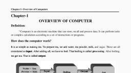
“Computing is not about computers anymore. It is about living. . . . We, have seen computers move out of giant air-conditioned rooms into, closets, then onto desktops, and now into our laps and pockets. But this, is not the end. . . . Like a force of nature, the digital age cannot be, denied or stopped. . . . The information superhighway may be mostly, hype today, but it is an understatement about tomorrow. It will exist, beyond people’s wildest predictions. . . . We are not waiting on any, invention. It is here. It is now. It is almost genetic in its nature, in that, each generation will become more digital than the preceding one.”, , —Nicholas Negroponte, professor of media technology at MIT, , CHAPTER, , 1, 1.1, , Introduction, , OVERVIEW, r. Negroponte is among many who see the computer revolution as if it were a, , Dforce of nature. This force has the potential to carry humanity to its digital, , destiny, allowing us to conquer problems that have eluded us for centuries, as, well as all of the problems that emerge as we solve the original problems. Computers have freed us from the tedium of routine tasks, liberating our collective, creative potential so that we can, of course, build bigger and better computers., As we observe the profound scientific and social changes that computers, have brought us, it is easy to start feeling overwhelmed by the complexity of it, all. This complexity, however, emanates from concepts that are fundamentally, very simple. These simple ideas are the ones that have brought us where we are, today, and are the foundation for the computers of the future. To what extent they, will survive in the future is anybody’s guess. But today, they are the foundation, for all of computer science as we know it., Computer scientists are usually more concerned with writing complex program algorithms than with designing computer hardware. Of course, if we want, our algorithms to be useful, a computer eventually has to run them. Some algorithms are so complicated that they would take too long to run on today’s systems. These kinds of algorithms are considered computationally infeasible., Certainly, at the current rate of innovation, some things that are infeasible today, could be feasible tomorrow, but it seems that no matter how big or fast computers, become, someone will think up a problem that will exceed the reasonable limits, of the machine., 1
Page 33 :
2, , Chapter 1 / Introduction, , To understand why an algorithm is infeasible, or to understand why the, implementation of a feasible algorithm is running too slowly, you must be able to, see the program from the computer’s point of view. You must understand what, makes a computer system tick before you can attempt to optimize the programs, that it runs. Attempting to optimize a computer system without first understanding it is like attempting to tune your car by pouring an elixir into the gas tank:, You’ll be lucky if it runs at all when you’re finished., Program optimization and system tuning are perhaps the most important, motivations for learning how computers work. There are, however, many other, reasons. For example, if you want to write compilers, you must understand the, hardware environment within which the compiler will function. The best compilers leverage particular hardware features (such as pipelining) for greater speed, and efficiency., If you ever need to model large, complex, real-world systems, you will need, to know how floating-point arithmetic should work as well as how it really works, in practice. If you wish to design peripheral equipment or the software that drives, peripheral equipment, you must know every detail of how a particular computer, deals with its input/output (I/O). If your work involves embedded systems, you, need to know that these systems are usually resource-constrained. Your understanding of time, space, and price tradeoffs, as well as I/O architectures, will be, essential to your career., All computer professionals should be familiar with the concepts of benchmarking and be able to interpret and present the results of benchmarking systems. People, who perform research involving hardware systems, networks, or algorithms find, benchmarking techniques crucial to their day-to-day work. Technical managers in, charge of buying hardware also use benchmarks to help them buy the best system, for a given amount of money, keeping in mind the ways in which performance, benchmarks can be manipulated to imply results favorable to particular systems., The preceding examples illustrate the idea that a fundamental relationship, exists between computer hardware and many aspects of programming and software components in computer systems. Therefore, regardless of our area of, expertise, as computer scientists, it is imperative that we understand how hardware interacts with software. We must become familiar with how various circuits, and components fit together to create working computer systems. We do this, through the study of computer organization. Computer organization addresses, issues such as control signals (how the computer is controlled), signaling methods, and memory types. It encompasses all physical aspects of computer systems., It helps us to answer the question: How does a computer work?, The study of computer architecture, on the other hand, focuses on the structure and behavior of the computer system and refers to the logical aspects of system implementation as seen by the programmer. Computer architecture includes, many elements such as instruction sets and formats, operation codes, data types,, the number and types of registers, addressing modes, main memory access methods, and various I/O mechanisms. The architecture of a system directly affects the, logical execution of programs. Studying computer architecture helps us to answer, the question: How do I design a computer?
Page 34 :
1.2 / The Main Components of a Computer, , 3, , The computer architecture for a given machine is the combination of its hardware components plus its instruction set architecture (ISA). The ISA is the, agreed-upon interface between all the software that runs on the machine and the, hardware that executes it. The ISA allows you to talk to the machine., The distinction between computer organization and computer architecture is, not clear-cut. People in the fields of computer science and computer engineering, hold differing opinions as to exactly which concepts pertain to computer organization and which pertain to computer architecture. In fact, neither computer, organization nor computer architecture can stand alone. They are interrelated and, interdependent. We can truly understand each of them only after we comprehend, both of them. Our comprehension of computer organization and architecture ultimately leads to a deeper understanding of computers and computation—the heart, and soul of computer science., , 1.2, , THE MAIN COMPONENTS OF A COMPUTER, Although it is difficult to distinguish between the ideas belonging to computer, organization and those ideas belonging to computer architecture, it is impossible, to say where hardware issues end and software issues begin. Computer scientists, design algorithms that usually are implemented as programs written in some, computer language, such as Java or C. But what makes the algorithm run?, Another algorithm, of course! And another algorithm runs that algorithm, and so, on until you get down to the machine level, which can be thought of as an algorithm implemented as an electronic device. Thus, modern computers are actually, implementations of algorithms that execute other algorithms. This chain of nested, algorithms leads us to the following principle:, Principle of Equivalence of Hardware and Software: Anything that, can be done with software can also be done with hardware, and anything, that can be done with hardware can also be done with software.1, A special-purpose computer can be designed to perform any task, such as word, processing, budget analysis, or playing a friendly game of Tetris. Accordingly,, programs can be written to carry out the functions of special-purpose computers,, such as the embedded systems situated in your car or microwave. There are times, when a simple embedded system gives us much better performance than a complicated computer program, and there are times when a program is the preferred, approach. The Principle of Equivalence of Hardware and Software tells us that, we have a choice. Our knowledge of computer organization and architecture will, help us to make the best choice., , 1What, , this principle does not address is the speed with which the equivalent tasks are carried out., Hardware implementations are almost always faster.
Page 35 :
4, , Chapter 1 / Introduction, , We begin our discussion of computer hardware by looking at the components, necessary to build a computing system. At the most basic level, a computer is a, device consisting of three pieces:, 1. A processor to interpret and execute programs, 2. A memory to store both data and programs, 3. A mechanism for transferring data to and from the outside world, We discuss these three components in detail as they relate to computer hardware, in the following chapters., Once you understand computers in terms of their component parts, you, should be able to understand what a system is doing at all times and how you, could change its behavior if so desired. You might even feel like you have a few, things in common with it. This idea is not as far-fetched as it appears. Consider, how a student sitting in class exhibits the three components of a computer: the, student’s brain is the processor, the notes being taken represent the memory, and, the pencil or pen used to take notes is the I/O mechanism. But keep in mind that, your abilities far surpass those of any computer in the world today, or any that, can be built in the foreseeable future., , 1.3, , AN EXAMPLE SYSTEM: WADING THROUGH THE JARGON, This book will introduce you to some of the vocabulary that is specific to computers. This jargon can be confusing, imprecise, and intimidating. We believe that, with a little explanation, we can clear the fog., For the sake of discussion, we have provided a facsimile computer advertisement (see Figure 1.1). The ad is typical of many in that it bombards the reader, with phrases such as “64MB SDRAM,” “64-bit PCI sound card” and “32KB L1, cache.” Without having a handle on such terminology, you would be hard-pressed, to know whether the stated system is a wise buy, or even whether the system is, able to serve your needs. As we progress through this book, you will learn the, concepts behind these terms., Before we explain the ad, however, we need to discuss something even more, basic: the measurement terminology you will encounter throughout your study of, computers., It seems that every field has its own way of measuring things. The computer, field is no exception. So that computer people can tell each other how big something is, or how fast something is, they must use the same units of measure. When, we want to talk about how big some computer thing is, we speak of it in terms of, thousands, millions, billions, or trillions of characters. The prefixes for terms are, given in the left side of Figure 1.2. In computing systems, as you shall see, powers of 2 are often more important than powers of 10, but it is easier for people to, understand powers of 10. Therefore, these prefixes are given in both powers of 10, and powers of 2. Because 1,000 is close in value to 210 (1,024), we can approximate powers of 10 by powers of 2. Prefixes used in system metrics are often, applied where the underlying base system is base 2, not base 10. For example, a
Page 36 :
1.3 / An Example System: Wading through the Jargon, , 5, , FOR SALE: OBSOLETE COMPUTER – CHEAP! CHEAP! CHEAP!, , • Pentium III 667 MHz, • 133 MHz 64MB SDRAM, • 32KB L1 cache, 256KB L2 cache, • 30GB EIDE hard drive (7200 RPM), • 48X max variable CD-ROM, • 2 USB ports, 1 serial port, 1 parallel port, • 19" monitor, .24mm AG, 1280 ⫻ 1024 at 85Hz, • Intel 3D AGP graphics card, • 56K PCI voice modem, • 64-bit PCI sound card, , FIGURE 1.1 A Typical Computer Advertisement, Kilo- (K), , (1 thousand = 103 ~, ~ 210), , Milli- (m), , –10, (1 thousandth = 10 –3 ~, ~2 ), , Mega- (M), , 20, (1 million = 106 ~, ~2 ), , Micro- (µ), , (1 millionth = 10–6 ~, ~ 2 –20), , Nano- (n), , (1 billionth = 10–9 ~ 2 –30), , Pico- (p), , (1 trillionth = 10–12 ~, ~ 2 –40), , Femto- (f), , (1 quadrillionth = 10–15 ~ 2 –50), , 109, , Giga- (G), , (1 billion =, , Tera- (T), , (1 trillion = 1012 ~, ~ 240), , Peta- (P), , (1 quadrillion =, , ~, , 230), , 1015, , ~, , 250), , FIGURE 1.2 Common Prefixes Associated with Computer Organization and, Architecture, , kilobyte (1KB) of memory is typically 1,024 bytes of memory rather than 1,000, bytes of memory. However, a 1GB disk drive might actually be 1 billion bytes, instead of 230 (approximately 1.7 billion). You should always read the manufacturer’s fine print just to make sure you know exactly what 1K, 1KB, or 1G represents., When we want to talk about how fast something is, we speak in terms of fractions of a second—usually thousandths, millionths, billionths, or trillionths. Prefixes for these metrics are given in the right-hand side of Figure 1.2. Notice that, the fractional prefixes have exponents that are the reciprocal of the prefixes on, the left side of the figure. Therefore, if someone says to you that an operation, requires a microsecond to complete, you should also understand that a million of, those operations could take place in one second. When you need to talk about, how many of these things happen in a second, you would use the prefix mega-., When you need to talk about how fast the operations are performed, you would, use the prefix micro-.
Page 37 :
6, , Chapter 1 / Introduction, , Now to explain the ad: The microprocessor is the part of a computer that, actually executes program instructions; it is the brain of the system. The microprocessor in the ad is a Pentium III, operating at 667MHz. Every computer system contains a clock that keeps the system synchronized. The clock sends, electrical pulses simultaneously to all main components, ensuring that data and, instructions will be where they’re supposed to be, when they’re supposed to be, there. The number of pulsations emitted each second by the clock is its frequency., Clock frequencies are measured in cycles per second, or hertz. Because computer, system clocks generate millions of pulses per second, we say that they operate in, the megahertz (MHz) range. Many computers today operate in the gigahertz, range, generating billions of pulses per second. And because nothing much gets, done in a computer system without microprocessor involvement, the frequency, rating of the microprocessor is crucial to overall system speed. The microprocessor of the system in our advertisement operates at 667 million cycles per second,, so the seller says that it runs at 667MHz., The fact that this microprocessor runs at 667MHz, however, doesn’t necessarily mean that it can execute 667 million instructions every second, or,, equivalently, that every instruction requires 1.5 nanoseconds to execute. Later, in this book, you will see that each computer instruction requires a fixed, number of cycles to execute. Some instructions require one clock cycle; however, most instructions require more than one. The number of instructions per, second that a microprocessor can actually execute is proportionate to its, clock speed. The number of clock cycles required to carry out a particular, machine instruction is a function of both the machine’s organization and its, architecture., The next thing that we see in the ad is “133MHz 64MB SDRAM.” The 133MHz, refers to the speed of the system bus, which is a group of wires that moves data and, instructions to various places within the computer. Like the microprocessor, the speed, of the bus is also measured in MHz. Many computers have a special local bus for data, that supports very fast transfer speeds (such as those required by video). This local, bus is a high-speed pathway that connects memory directly to the processor. Bus, speed ultimately sets the upper limit on the system’s information-carrying capability., The system in our advertisement also boasts a memory capacity of 64, megabytes (MB), or about 64 million characters. Memory capacity not only, determines the size of the programs that you can run, but also how many programs you can run at the same time without bogging down the system. Your, application or operating system manufacturer will usually recommend how much, memory you’ll need to run their products. (Sometimes these recommendations, can be hilariously conservative, so be careful whom you believe!), In addition to memory size, our advertised system provides us with a memory, type, SDRAM, short for synchronous dynamic random access memory. SDRAM, is much faster than conventional (nonsynchronous) memory because it can synchronize itself with a microprocessor’s bus. At this writing, SDRAM bus synchronization is possible only with buses running at 200MHz and below. Newer, memory technologies such as RDRAM (Rambus DRAM) and SLDRAM, (SyncLink DRAM) are required for systems running faster buses.
Page 38 :
1.3 / An Example System: Wading through the Jargon, , A Look Inside a Computer, Have you even wondered what the inside of a computer really looks like? The, example computer described in this section gives a good overview of the components of a modern PC. However, opening a computer and attempting to find, and identify the various pieces can be frustrating, even if you are familiar with, the components and their functions., , Courtesy of Intel Corporation, , If you remove the cover on your computer, you will no doubt first notice a, big metal box with a fan attached. This is the power supply. You will also see, various drives, including a hard drive, and perhaps a floppy drive and CD-ROM, or DVD drive. There are many integrated circuits — small, black rectangular, boxes with legs attached. You will also notice electrical pathways, or buses, in, the system. There are printed circuit boards (expansion cards) that plug into, sockets on the motherboard, the large board at the bottom of a standard desktop PC or on the side of a PC configured as a tower or mini-tower. The motherboard is the printed circuit board that connects all of the components in the, , 7
Page 39 :
8, , Chapter 1 / Introduction, , computer, including the CPU, and RAM and ROM memory, as well as an assortment of other essential components. The components on the motherboard, tend to be the most difficult to identify. Above you see an Intel D850 motherboard with the more important components labeled., The I/O ports at the top of the board allow the computer to communicate, with the outside world. The I/O controller hub allows all connected devices to, function without conflict. The PCI slots allow for expansion boards belonging to, various PCI devices. The AGP connector is for plugging in the AGP graphics card., There are two RAM memory banks and a memory controller hub. There is no, processor plugged into this motherboard, but we see the socket where the CPU, is to be placed. All computers have an internal battery, as seen at the lower lefthand corner. This motherboard has two IDE connector slots, and one floppy disk, controller. The power supply plugs into the power connector., A note of caution regarding looking inside the box: There are many safety, considerations involved with removing the cover for both you and your computer. There are many things you can do to minimize the risks. First and foremost, make sure the computer is turned off. Leaving it plugged in is often, preferred, as this offers a path for static electricity. Before opening your computer and touching anything inside, you should make sure you are properly, grounded so static electricity will not damage any components. Many of the, edges, both on the cover and on the circuit boards, can be sharp, so take care, when handling the various pieces. Trying to jam misaligned cards into sockets, can damage both the card and the motherboard, so be careful if you decide to, add a new card or remove and reinstall an existing one., , The next line in the ad, “32KB L1 cache, 256KB L2 cache” also, describes a type of memory. In Chapter 6, you will learn that no matter how, fast a bus is, it still takes “a while” to get data from memory to the processor., To provide even faster access to data, many systems contain a special memory called cache. The system in our advertisement has two kinds of cache., Level 1 cache (L1) is a small, fast memory cache that is built into the microprocessor chip and helps speed up access to frequently used data. Level 2, cache (L2) is a collection of fast, built-in memory chips situated between the, microprocessor and main memory. Notice that the cache in our system has a, capacity of kilobytes (KB), which is much smaller than main memory. In, Chapter 6 you will learn how cache works, and that a bigger cache isn’t, always better., On the other hand, everyone agrees that the more fixed disk capacity you, have, the better off you are. The advertised system has 30GB, which is fairly, impressive. The storage capacity of a fixed (or hard) disk is not the only thing to, consider, however. A large disk isn’t very helpful if it is too slow for its host system. The computer in our ad has a hard drive that rotates at 7200 RPM (revolutions per minute). To the knowledgeable reader, this indicates (but does not state
Page 40 :
1.3 / An Example System: Wading through the Jargon, , 9, , outright) that this is a fairly fast drive. Usually disk speeds are stated in terms of, the number of milliseconds required (on average) to access data on the disk, in, addition to how fast the disk rotates., Rotational speed is only one of the determining factors in the overall performance of a disk. The manner in which it connects to—or interfaces with—the, rest of the system is also important. The advertised system uses a disk interface, called EIDE, or enhanced integrated drive electronics. EIDE is a cost-effective, hardware interface for mass storage devices. EIDE contains special circuits that, allow it to enhance a computer’s connectivity, speed, and memory capability., Most EIDE systems share the main system bus with the processor and memory,, so the movement of data to and from the disk is also dependent on the speed of, the system bus., Whereas the system bus is responsible for all data movement internal to, the computer, ports allow movement of data to and from devices external to, the computer. Our ad speaks of three different ports with the line, “2 USB, ports, 1 serial port, 1 parallel port.” Most desktop computers come with two, kinds of data ports: serial ports and parallel ports. Serial ports transfer data by, sending a series of electrical pulses across one or two data lines. Parallel ports, use at least eight data lines, which are energized simultaneously to transmit, data. Our advertised system also comes equipped with a special serial connection called a USB (universal serial bus) port. USB is a popular external bus, that supports Plug-and-Play (the ability to configure devices automatically) as, well as hot plugging (the ability to add and remove devices while the computer, is running)., Some systems augment their main bus with dedicated I/O buses. Peripheral, Component Interconnect (PCI) is one such I/O bus that supports the connection, of multiple peripheral devices. PCI, developed by the Intel Corporation, operates at high speeds and also supports Plug-and-Play. There are two PCI devices, mentioned in the ad. The PCI modem allows the computer to connect to the, Internet. (We discuss modems in detail in Chapter 11.) The other PCI device is a, sound card, which contains components needed by the system’s stereo speakers., You will learn more about different kinds of I/O, I/O buses, and disk storage in, Chapter 7., After telling us about the ports in the advertised system, the ad supplies us, with some specifications for the monitor by saying, “19" monitor, .24mm AG,, 1280 ⫻ 1024 at 85Hz.” Monitors have little to do with the speed or efficiency of, a computer system, but they have great bearing on the comfort of the user. The, monitor in the ad supports a refresh rate of 85Hz. This means that the image displayed on the monitor is repainted 85 times a second. If the refresh rate is too, slow, the screen may exhibit an annoying jiggle or wavelike behavior. The eyestrain caused by a wavy display makes people tire easily; some people may even, experience headaches after periods of prolonged use. Another source of eyestrain, is poor resolution. A higher-resolution monitor makes for better viewing and finer, graphics. Resolution is determined by the dot pitch of the monitor, which is the, distance between a dot (or pixel) and the closest dot of the same color. The, smaller the dot, the sharper the image. In this case, we have a 0.28 millimeter
Page 41 :
10, , Chapter 1 / Introduction, , (mm) dot pitch supported by an AG (aperture grill) display. Aperture grills direct, the electron beam that paints the monitor picture on the phosphor coating inside, the glass of the monitor. AG monitors produce crisper images than the older, shadow mask technology. This monitor is further supported by an AGP (accelerated graphics port) graphics card. This is a graphics interface designed by Intel, specifically for 3D graphics., In light of the preceding discussion, you may be wondering why monitor dot, pitch can’t be made arbitrarily small to give picture perfect resolution. The reason, is that the refresh rate is dependent on the dot pitch. Refreshing 100 dots, for, example, requires more time than refreshing 50 dots. A smaller dot pitch requires, more dots to cover the screen. The more dots to refresh, the longer it takes for, each refresh cycle. Experts recommend a refresh rate of at least 75Hz. The 85Hz, refresh rate of the advertised monitor is better than the minimum recommendation by 10Hz (about 13%)., Although we cannot delve into all of the brand-specific components available, after completing this book, you should understand the concept of how, most computer systems operate. This understanding is important for casual, users as well as experienced programmers. As a user, you need to be aware of, the strengths and limitations of your computer system so you can make, informed decisions about applications and thus use your system more effectively. As a programmer, you need to understand exactly how your system, hardware functions so you can write effective and efficient programs. For, example, something as simple as the algorithm your hardware uses to map, main memory to cache and the method used for memory interleaving can have, a tremendous impact on your decision to access array elements in row versus, column-major order., Throughout this book, we investigate both large and small computers. Large, computers include mainframes (enterprise-class servers) and supercomputers., Small computers include personal systems, workstations and handheld devices., We will show that regardless of whether they carry out routine chores or perform, sophisticated scientific tasks, the components of these systems are very similar., We also visit some architectures that lie outside what is now the mainstream of, computing. We hope that the knowledge that you gain from this book will ultimately serve as a springboard for your continuing studies within the vast and, exciting fields of computer organization and architecture., , 1.4, , STANDARDS ORGANIZATIONS, Suppose you decide that you’d like to have one of those nifty new .28mm dot, pitch AG monitors. You figure that you can shop around a bit to find the best, price. You make a few phone calls, surf the Web, and drive around town until you, find the one that gives you the most for your money. From your experience, you, know that you can buy your monitor anywhere and it will probably work fine on, your system. You can make this assumption because computer equipment manu-
Page 42 :
1.4 / Standards Organizations, , 11, , facturers have agreed to comply with connectivity and operational specifications, established by a number of government and industry organizations., Some of these standards-setting organizations are ad-hoc trade associations, or consortia made up of industry leaders. Manufacturers know that by establishing common guidelines for a particular type of equipment, they can market their, products to a wider audience than if they came up with separate—and perhaps, incompatible—specifications., Some standards organizations have formal charters and are recognized internationally as the definitive authority in certain areas of electronics and computers. As you continue your studies in computer organization and architecture, you, will encounter specifications formulated by these groups, so you should know, something about them., The Institute of Electrical and Electronic Engineers (IEEE) is an organization, dedicated to the advancement of the professions of electronic and computer engineering. The IEEE actively promotes the interests of the worldwide engineering, community by publishing an array of technical literature. The IEEE also sets standards for various computer components, signaling protocols, and data representation,, to name only a few areas of its involvement. The IEEE has a democratic, albeit convoluted, procedure established for the creation of new standards. Its final documents, are well respected and usually endure for several years before requiring revision., The International Telecommunications Union (ITU) is based in Geneva,, Switzerland. The ITU was formerly known as the Comité Consultatif International, Télégraphique et Téléphonique, or the International Consultative Committee on, Telephony and Telegraphy. As its name implies, the ITU concerns itself with the, interoperability of telecommunications systems, including telephone, telegraph, and, data communication systems. The telecommunications arm of the ITU, the ITU-T,, has established a number of standards that you will encounter in the literature. You, will see these standards prefixed by ITU-T or the group’s former initials, CCITT., Many countries, including the European Community, have commissioned, umbrella organizations to represent their interests within various international, groups. The group representing the United States is the American National Standards Institute (ANSI). Great Britain has its British Standards Institution (BSI) in, addition to having a voice on CEN (Comite Europeen de Normalisation), the, European committee for standardization., The International Organization for Standardization (ISO) is the entity that, coordinates worldwide standards development, including the activities of ANSI, with BSI among others. ISO is not an acronym, but derives from the Greek word,, isos, meaning “equal.” The ISO consists of over 2,800 technical committees, each, of which is charged with some global standardization issue. Its interests range, from the behavior of photographic film to the pitch of screw threads to the complex world of computer engineering. The proliferation of global trade has been, facilitated by the ISO. Today, the ISO touches virtually every aspect of our lives., Throughout this book, we mention official standards designations where, appropriate. Definitive information concerning many of these standards can be
Page 43 :
12, , Chapter 1 / Introduction, , found in excruciating detail on the Web site of the organization responsible for, establishing the standard cited. As an added bonus, many standards contain “normative” and informative references, which provide background information in, areas related to the standard., , 1.5, , HISTORICAL DEVELOPMENT, During their 50-year life span, computers have become the perfect example of, modern convenience. Living memory is strained to recall the days of steno, pools, carbon paper, and mimeograph machines. It sometimes seems that, these magical computing machines were developed instantaneously in the, form that we now know them. But the developmental path of computers is, paved with accidental discovery, commercial coercion, and whimsical fancy., And occasionally computers have even improved through the application of, solid engineering practices! Despite all of the twists, turns, and technological, dead ends, computers have evolved at a pace that defies comprehension. We, can fully appreciate where we are today only when we have seen where we’ve, come from., In the sections that follow, we divide the evolution of computers into generations, each generation being defined by the technology used to build the machine., We have provided approximate dates for each generation for reference purposes, only. You will find little agreement among experts as to the exact starting and, ending times of each technological epoch., Every invention reflects the time in which it was made, so one might wonder whether it would have been called a computer if it had been invented in the, late 1990s. How much computation do we actually see pouring from the mysterious boxes perched on or beside our desks? Until recently, computers served us, only by performing mind-bending mathematical manipulations. No longer limited to white-jacketed scientists, today’s computers help us to write documents,, keep in touch with loved ones across the globe, and do our shopping chores., Modern business computers spend only a minuscule part of their time performing accounting calculations. Their main purpose is to provide users with a, bounty of strategic information for competitive advantage. Has the word computer now become a misnomer? An anachronism? What, then, should we call, them, if not computers?, We cannot present the complete history of computing in a few pages. Entire, books have been written on this subject and even they leave their readers wanting, for more detail. If we have piqued your interest, we refer you to look at some of, the books cited in the list of references at the end of this chapter., , 1.5.1, , Generation Zero: Mechanical Calculating Machines (1642–1945), Prior to the 1500s, a typical European businessperson used an abacus for calculations and recorded the result of his ciphering in Roman numerals. After the, decimal numbering system finally replaced Roman numerals, a number of people invented devices to make decimal calculations even faster and more accu-
Page 44 :
1.5 / Historical Development, , 13, , rate. Wilhelm Schickard (1592–1635) has been credited with the invention of the, first mechanical calculator, the Calculating Clock (exact date unknown). This, device was able to add and subtract numbers containing as many as six digits. In, 1642, Blaise Pascal (1623–1662) developed a mechanical calculator called the, Pascaline to help his father with his tax work. The Pascaline could do addition, with carry and subtraction. It was probably the first mechanical adding device, actually used for a practical purpose. In fact, the Pascaline was so well conceived that its basic design was still being used at the beginning of the twentieth, century, as evidenced by the Lightning Portable Adder in 1908, and the Addometer in 1920. Gottfried Wilhelm von Leibniz (1646–1716), a noted mathematician, invented a calculator known as the Stepped Reckoner that could add,, subtract, multiply, and divide. None of these devices could be programmed or, had memory. They required manual intervention throughout each step of their, calculations., Although machines like the Pascaline were used into the twentieth century,, new calculator designs began to emerge in the nineteenth century. One of the, most ambitious of these new designs was the Difference Engine by Charles Babbage (1791–1871). Some people refer to Babbage as “the father of computing.”, By all accounts, he was an eccentric genius who brought us, among other things,, the skeleton key and the “cow catcher,” a device intended to push cows and other, movable obstructions out of the way of locomotives., Babbage built his Difference Engine in 1822. The Difference Engine got its, name because it used a calculating technique called the method of differences. The, machine was designed to mechanize the solution of polynomial functions and was, actually a calculator, not a computer. Babbage also designed a general-purpose, machine in 1833 called the Analytical Engine. Although Babbage died before he, could build it, the Analytical Engine was designed to be more versatile than his, earlier Difference Engine. The Analytical Engine would have been capable of performing any mathematical operation. The Analytical Engine included many of the, components associated with modern computers: an arithmetic processing unit to, perform calculations (Babbage referred to this as the mill), a memory (the store),, and input and output devices. Babbage also included a conditional branching, operation where the next instruction to be performed was determined by the result, of the previous operation. Ada, Countess of Lovelace and daughter of poet Lord, Byron, suggested that Babbage write a plan for how the machine would calculate, numbers. This is regarded as the first computer program, and Ada is considered to, be the first computer programmer. It is also rumored that she suggested the use of, the binary number system rather than the decimal number system to store data., A perennial problem facing machine designers has been how to get data into, the machine. Babbage designed the Analytical Engine to use a type of punched, card for input and programming. Using cards to control the behavior of a machine, did not originate with Babbage, but with one of his friends, Joseph-Marie, Jacquard (1752–1834). In 1801, Jacquard invented a programmable weaving, loom that could produce intricate patterns in cloth. Jacquard gave Babbage a tapestry that had been woven on this loom using more than 10,000 punched cards., To Babbage, it seemed only natural that if a loom could be controlled by cards,
Page 45 :
14, , Chapter 1 / Introduction, , then his Analytical Engine could be as well. Ada expressed her delight with this, idea, writing, “[T]he Analytical Engine weaves algebraical patterns just as the, Jacquard loom weaves flowers and leaves.”, The punched card proved to be the most enduring means of providing input to a, computer system. Keyed data input had to wait until fundamental changes were, made in how calculating machines were constructed. In the latter half of the nineteenth century, most machines used wheeled mechanisms, which were difficult to, integrate with early keyboards because they were levered devices. But levered, devices could easily punch cards and wheeled devices could easily read them. So a, number of devices were invented to encode and then “tabulate” card-punched data., The most important of the late-nineteenth-century tabulating machines was the one, invented by Herman Hollerith (1860–1929). Hollerith’s machine was used for, encoding and compiling 1890 census data. This census was completed in record, time, thus boosting Hollerith’s finances and the reputation of his invention. Hollerith, later founded the company that would become IBM. His 80-column punched card,, the Hollerith card, was a staple of automated data processing for over 50 years., 1.5.2, , The First Generation: Vacuum Tube Computers (1945–1953), Although Babbage is often called the “father of computing,” his machines were, mechanical, not electrical or electronic. In the 1930s, Konrad Zuse (1910–1995), picked up where Babbage left off, adding electrical technology and other improvements to Babbage’s design. Zuse’s computer, the Z1, used electromechanical, relays instead of Babbage’s hand-cranked gears. The Z1 was programmable and, had a memory, an arithmetic unit, and a control unit. Because money and resources, were scarce in wartime Germany, Zuse used discarded movie film instead of, punched cards for input. Although his machine was designed to use vacuum tubes,, Zuse, who was building his machine on his own, could not afford the tubes. Thus,, the Z1 correctly belongs in the first generation, although it had no tubes., Zuse built the Z1 in his parents’ Berlin living room while Germany was at, war with most of Europe. Fortunately, he couldn’t convince the Nazis to buy his, machine. They did not realize the tactical advantage such a device would give, them. Allied bombs destroyed all three of Zuse’s first systems, the Z1, Z2, and, Z3. Zuse’s impressive machines could not be refined until after the war and ended, up being another “evolutionary dead end” in the history of computers., Digital computers, as we know them today, are the outcome of work done by, a number of people in the 1930s and 1940s. Pascal’s basic mechanical calculator, was designed and modified simultaneously by many people; the same can be said, of the modern electronic computer. Notwithstanding the continual arguments, about who was first with what, three people clearly stand out as the inventors of, modern computers: John Atanasoff, John Mauchly, and J. Presper Eckert., John Atanasoff (1904–1995) has been credited with the construction of the, first completely electronic computer. The Atanasoff Berry Computer (ABC) was, a binary machine built from vacuum tubes. Because this system was built specifi-
Page 46 :
1.5 / Historical Development, , 15, , cally to solve systems of linear equations, we cannot call it a general-purpose, computer. There were, however, some features that the ABC had in common with, the general-purpose ENIAC (Electronic Numerical Integrator and Computer),, which was invented a few years later. These common features caused considerable controversy as to who should be given the credit (and patent rights) for the, invention of the electronic digital computer. (The interested reader can find more, details on a rather lengthy lawsuit involving Atanasoff and the ABC in Mollenhoff [1988].), John Mauchly (1907–1980) and J. Presper Eckert (1929–1995) were the two, principle inventors of the ENIAC, introduced to the public in 1946. The ENIAC, is recognized as the first all-electronic, general-purpose digital computer. This, machine used 17,468 vacuum tubes, occupied 1,800 square feet of floor space,, weighed 30 tons, and consumed 174 kilowatts of power. The ENIAC had a memory capacity of about 1,000 information bits (about 20 10-digit decimal numbers), and used punched cards to store data., John Mauchly’s vision for an electronic calculating machine was born from, his lifelong interest in predicting the weather mathematically. While a professor, of physics at Ursinus College near Philadelphia, Mauchly engaged dozens of, adding machines and student operators to crunch mounds of data that he believed, would reveal mathematical relationships behind weather patterns. He felt that if, he could have only a little more computational power, he could reach the goal, that seemed just beyond his grasp. Pursuant to the Allied war effort, and with, ulterior motives to learn about electronic computation, Mauchly volunteered for a, crash course in electrical engineering at the University of Pennsylvania’s Moore, School of Engineering. Upon completion of this program, Mauchly accepted a, teaching position at the Moore School, where he taught a brilliant young student,, J. Presper Eckert. Mauchly and Eckert found a mutual interest in building an, electronic calculating device. In order to secure the funding they needed to build, their machine, they wrote a formal proposal for review by the school. They portrayed their machine as conservatively as they could, billing it as an “automatic, calculator.” Although they probably knew that computers would be able to function most efficiently using the binary numbering system, Mauchly and Eckert, designed their system to use base 10 numbers, in keeping with the appearance of, building a huge electronic adding machine. The university rejected Mauchly and, Eckert’s proposal. Fortunately, the United States Army was more interested., During World War II, the army had an insatiable need for calculating the trajectories of its new ballistic armaments. Thousands of human “computers” were, engaged around the clock cranking through the arithmetic required for these firing, tables. Realizing that an electronic device could shorten ballistic table calculation, from days to minutes, the army funded the ENIAC. And the ENIAC did indeed, shorten the time to calculate a table from 20 hours to 30 seconds. Unfortunately,, the machine wasn’t ready before the end of the war. But the ENIAC had shown, that vacuum tube computers were fast and feasible. During the next decade, vacuum tube systems continued to improve and were commercially successful.
Page 47 :
16, , Chapter 1 / Introduction, , U.S. Army, 1946
Page 48 :
1.5 / Historical Development, , 17, , What Is a Vacuum Tube?, , Plate, (Anode), Control, Grid, Cathode, Envelope, , The wired world that we know today was born from the invention of a single, electronic device called a vacuum tube by Americans and—more accurately—a, valve by the British. Vacuum tubes should be called valves because, they control the flow of electrons in electrical systems in much the, same way as valves control the flow of water in a plumbing system. In fact, some mid-twentieth-century breeds of these electron, tubes contain no vacuum at all, but are filled with conductive, gasses, such as mercury vapor, which can provide desirable electrical behavior., The electrical phenomenon that makes tubes work was discovered by Thomas A. Edison in 1883 while he was trying to, find ways to keep the filaments of his light bulbs from burning, away (or oxidizing) a few minutes after electrical current was, applied. Edison reasoned correctly that one way to prevent filament oxidation would be to place the filament in a vacuum. Edison didn’t immediately understand that air not only supports, combustion, but also is a good insulator. When he energized the electrodes, holding a new tungsten filament, the filament soon became hot and burned, out as the others had before it. This time, however, Edison noticed that, electricity continued to flow from the warmed negative terminal to the cool, positive terminal within the light bulb. In 1911, Owen Willans Richardson, analyzed this behavior. He concluded that when a negatively charged filament was heated, electrons “boiled off” as water molecules can be boiled to, create steam. He aptly named this phenomenon thermionic emission., Thermionic emission, as Edison had documented it, was thought by many, to be only an electrical curiosity. But in 1905 a British former assistant to Edison, John A. Fleming, saw Edison’s discovery as much more than a novelty. He, knew that thermionic emission supported the flow of electrons in only one, direction: from the negatively charged cathode to the positively charged anode,, also called a plate. He realized that this behavior could rectify alternating current. That is, it could change alternating current into the direct current that, was essential for the proper operation of telegraph equipment. Fleming used, his ideas to invent an electronic valve later called a diode tube or rectifier., , +, –, , Rectifier, , The diode was well suited for changing alternating current into direct current, but the greatest power of the electron tube was yet to be discovered. In
Page 49 :
18, , Chapter 1 / Introduction, , 1907, an American named Lee DeForest added a third element, called a control, grid. The control grid, when carrying a negative charge, can reduce or prevent, electron flow from the cathode to the anode of a diode., Negative charge, on cathode and control, grid; positive on anode:, Electrons stay near, cathode., , Negative charge on, cathode; positive on, control grid and anode:, Electrons travel from, cathode to anode., , +, , –, –, , Filament, , Diode, , Tetrode, , +, , –, , +, , When DeForest patented his device, he called it an audion tube. It was later, known as a triode. The schematic symbol for the triode is shown at the left., A triode can act either as a switch or as an amplifier. Small changes, Grid, in the charge of the control grid can cause much larger changes in the, flow of electrons between the cathode and the anode. Therefore, a, weak signal applied to the grid results in a much stronger signal at the, plate output. A sufficiently large negative charge applied to the grid, Anode, (plate), stops all electrons from leaving the cathode., Cathode, Additional control grids were eventually added to the triode to allow, more exact control of the electron flow. Tubes with two grids (four elements) are called tetrodes; tubes with three grids are called pentodes. Triodes, and pentodes were the tubes most commonly used in communications and computer applications. Often, two or three triodes or pentodes would be combined, within one envelope so that they could share a single heater, thereby reducing, the power consumption of a particular device. These latter-day devices were, called “miniature” tubes because many were about 2 inches (5cm), high and one-half inch (1.5cm) in diameter. Equivalent full-sized, diodes, triodes, and pentodes were just a little smaller than a, household light bulb., Vacuum tubes were not well suited for building computers., Even the simplest vacuum tube computer system required thouTriode, sands of tubes. Enormous amounts of electrical power were, required to heat the cathodes of these devices. To prevent a meltdown, this heat had to be removed from the system as quickly as, possible. Power consumption and heat dissipation could be, reduced by running the cathode heaters at lower voltages, but this, reduced the already slow switching speed of the tube. Despite, their limitations and power consumption, vacuum tube computer, Pentode
Page 50 :
1.5 / Historical Development, , 19, , systems, both analog and digital, served their purpose for many years and are the, architectural foundation for all modern computer systems., Although decades have passed since the last vacuum tube computer was, manufactured, vacuum tubes are still used in audio amplifiers. These “high-end”, amplifiers are favored by musicians who believe that tubes provide a resonant, and pleasing sound unattainable by solid-state devices., , 1.5.3, , The Second Generation: Transistorized Computers (1954–1965), The vacuum tube technology of the first generation was not very dependable. In, fact, some ENIAC detractors believed that the system would never run because, the tubes would burn out faster than they could be replaced. Although system reliability wasn’t as bad as the doomsayers predicted, vacuum tube systems often, experienced more downtime than uptime., In 1948, three researchers with Bell Laboratories—John Bardeen, Walter Brattain, and William Shockley—invented the transistor. This new technology not only, revolutionized devices such as televisions and radios, but also pushed the computer, industry into a new generation. Because transistors consume less power than vacuum, tubes, are smaller, and work more reliably, the circuitry in computers consequently, became smaller and more reliable. Despite using transistors, computers of this generation were still bulky and quite costly. Typically only universities, governments, and, large businesses could justify the expense. Nevertheless, a plethora of computer, makers emerged in this generation; IBM, Digital Equipment Corporation (DEC),, and Univac (now Unisys) dominated the industry. IBM marketed the 7094 for scientific applications and the 1401 for business applications. DEC was busy manufacturing the PDP-1. A company founded (but soon sold) by Mauchly and Eckert built the, Univac systems. The most successful Unisys systems of this generation belonged to, its 1100 series. Another company, Control Data Corporation (CDC), under the supervision of Seymour Cray, built the CDC 6600, the world’s first supercomputer. The, $10 million CDC 6600 could perform 10 million instructions per second, used 60-bit, words, and had an astounding 128 kilowords of main memory., , What Is a Transistor?, The transistor, short for transfer resistor, is the solid-state version of the triode., There is no such thing as a solid-state version of the tetrode or pentode. Because, electrons are better behaved in a solid medium than in the open void of a vacuum, tube, they need no extra controlling grids. Either germanium or silicon can be the, basic “solid” used in these solid state devices. In their pure form, neither of these, elements is a good conductor of electricity. But when they are combined with
Page 51 :
20, , Chapter 1 / Introduction, , A few, electrons, withdrawn, , –, , trace amounts of elements that are their neighbors in the Periodic Chart, of the Elements, they conduct electricity in an effective and easily controlled manner., Boron, aluminum, and gallium can be found to the left of silicon, and germanium on the Periodic Chart. Because they lie to the left of silicon and germanium, they have one less electron in their outer electron, shell, or valence. So if you add a small amount of aluminum to silicon,, the silicon ends up with a slight imbalance in its outer electron shell,, and therefore attracts electrons from any pole that has a negative, potential (an excess of electrons). When modified (or doped) in this, way, silicon or germanium becomes a P-type material., Similarly, if we add a little boron, arsenic, or, gallium to silicon, we’ll have extra electrons in, valences of the silicon crystals. This gives us an Ntype material. A small amount of current will flow, through the N-type material if we provide the, Emitter, loosely bound electrons in the N-type material with, Base, a place to go. In other words, if we apply a positive, Collector, potential to N-type material, electrons will flow, from the negative pole to the positive pole. If the, poles are reversed, that is, if we apply a negative potential to the N-type material and a positive potential to the P-type material, no current will flow. This, means that we can make a solid-state diode from a simple junction of N- and, P-type materials., The solid-state triode, the transistor, consists of three layers of semiconductor material. Either a slice of P-type material is sandwiched between two N-type, materials, or a slice of N-type material is sandwiched between two P-type materials. The former is called an NPN transistor, the latter a PNP transistor. The, inner layer of the transistor is called the base; the other two layers are called the, collector and emitter., The figure to the left shows how current flows through NPN and PNP transistors. The base in a transistor works just like the control grid in a triode tube:, Small changes in the current at the base of a transistor result in a large electron, flow from the emitter to the collector., A discrete-component transistor is shown in, Electron Source, “TO-50” packaging in the figure at the beginning, of this sidebar. There are only three wires (leads), A few, that connect the base, emitter, and collector of, electrons, the transistor to the rest of the circuit. Transistors, added, are not only smaller than vacuum tubes, but they, also run cooler and are much more reliable. Vacuum tube filaments, like light bulb filaments, run, Large, hot and eventually burn out. Computers using, current output, + transistorized components will naturally be
Page 52 :
1.5 / Historical Development, , smaller and run cooler than their vacuum tube predecessors. The ultimate miniaturization, however, is not, realized by replacing individual triodes with discrete, N, transistors, but in shrinking entire circuits onto one, Base, P, piece of silicon., N, Collector, Integrated circuits, or chips, contain hundreds to, millions of microscopic transistors. Several different, techniques are used to manufacture integrated circuits. One of the simplest methods involves creating a circuit using computeraided design software that can print large maps of each of the several silicon layers, forming the chip. Each map is used like a photographic negative where lightinduced changes in a photoresistive substance on the chip’s surface produce the, delicate patterns of the circuit when the silicon chip is immersed in a chemical that, washes away the exposed areas of the silicon. This technique is called photomicrolithography. After the etching is completed, a layer of N-type or P-type material, is deposited on the bumpy surface of the chip. This layer is then treated with a, photoresistive substance, exposed to light, and etched as was the layer before it., This process continues until all of the layers have been etched. The resulting peaks, and valleys of P- and N-material form microscopic electronic components, including transistors, that behave just like larger versions fashioned from discrete components, except that they run a lot faster and consume a small fraction of the power., , Emitter, , N, P, N, , 1.5.4, , 21, , Contacts, , The Third Generation: Integrated Circuit Computers (1965–1980), The real explosion in computer use came with the integrated circuit generation., Jack Kilby invented the integrated circuit (IC) or microchip, made of germanium., Six months later, Robert Noyce (who had also been working on integrated circuit, design) created a similar device using silicon instead of germanium. This is the, silicon chip upon which the computer industry was built. Early ICs allowed, dozens of transistors to exist on a single silicon chip that was smaller than a single “discrete component” transistor. Computers became faster, smaller, and, cheaper, bringing huge gains in processing power. The IBM System/360 family, of computers was among the first commercially available systems to be built, entirely of solid-state components. The 360 product line was also IBM’s first, offering where all of the machines in the family were compatible, meaning they, all used the same assembly language. Users of smaller machines could upgrade to, larger systems without rewriting all of their software. This was a revolutionary, new concept at the time., The IC generation also saw the introduction of time-sharing and multiprogramming (the ability for more than one person to use the computer at a time)., Multiprogramming, in turn, necessitated the introduction of new operating systems for these computers. Time-sharing minicomputers such as DEC’s PDP-8 and, PDP-11 made computing affordable to smaller businesses and more universities.
Page 53 :
22, , Chapter 1 / Introduction, , Comparison of Computer Components, Clockwise, starting from the top:, 1) Vacuum Tube, 2) Transistor, 3) Chip containing 3200 2-input NAND gates, 4) Integrated circuit package (the small silver square in, the lower left-hand corner is an integrated circuit), Courtesy of Linda Null, , IC technology also allowed for the development of more powerful supercomputers. Seymour Cray took what he had learned while building the CDC 6600 and, started his own company, the Cray Research Corporation. This company produced a number of supercomputers, starting with the $8.8 million Cray-1, in, 1976. The Cray-1, in stark contrast to the CDC 6600, could execute over 160 million instructions per second and could support 8 megabytes of memory., 1.5.5, , The Fourth Generation: VLSI Computers (1980–????), In the third generation of electronic evolution, multiple transistors were integrated onto one chip. As manufacturing techniques and chip technologies, advanced, increasing numbers of transistors were packed onto one chip. There are, now various levels of integration: SSI (small scale integration), in which there are
Page 54 :
1.5 / Historical Development, , 23, , 10 to 100 components per chip; MSI (medium scale integration), in which there, are 100 to 1,000 components per chip; LSI (large scale integration), in which, there are 1,000 to 10,000 components per chip; and finally, VLSI (very large, scale integration), in which there are more than 10,000 components per chip. This, last level, VLSI, marks the beginning of the fourth generation of computers., To give some perspective to these numbers, consider the ENIAC-on-a-chip, project. In 1997, to commemorate the fiftieth anniversary of its first public, demonstration, a group of students at the University of Pennsylvania constructed, a single-chip equivalent of the ENIAC. The 1,800 square-foot, 30-ton beast that, devoured 174 kilowatts of power the minute it was turned on had been reproduced on a chip the size of a thumbnail. This chip contained approximately, 174,569 transistors—an order of magnitude fewer than the number of components typically placed on the same amount of silicon in the late 1990s., VLSI allowed Intel, in 1971, to create the world’s first microprocessor, the, 4004, which was a fully functional, 4-bit system that ran at 108KHz. Intel also, introduced the random access memory (RAM) chip, accommodating four kilobits, of memory on a single chip. This allowed computers of the fourth generation to, become smaller and faster than their solid-state predecessors., VLSI technology, and its incredible shrinking circuits, spawned the development of microcomputers. These systems were small enough and inexpensive, enough to make computers available and affordable to the general public. The, premiere microcomputer was the Altair 8800, released in 1975 by the Micro, Instrumentation and Telemetry (MITS) corporation. The Altair 8800 was soon, followed by the Apple I and Apple II, and Commodore’s PET and Vic 20. Finally,, in 1981, IBM introduced its PC (Personal Computer)., The Personal Computer was IBM’s third attempt at producing an “entry-level”, computer system. Its Datamaster as well as its 5100 Series desktop computers, flopped miserably in the marketplace. Despite these early failures, IBM’s John Opel, convinced his management to try again. He suggested forming a fairly autonomous, “independent business unit” in Boca Raton, Florida, far from IBM’s headquarters in, Armonk, New York. Opel picked Don Estridge, an energetic and capable engineer,, to champion the development of the new system, code-named the Acorn. In light of, IBM’s past failures in the small-systems area, corporate management held tight rein, on the Acorn’s timeline and finances. Opel could get his project off of the ground, only after promising to deliver it within a year, a seemingly impossible feat., Estridge knew that the only way that he could deliver the PC within the, wildly optimistic 12-month schedule would be to break with IBM convention and, use as many “off-the-shelf” parts as possible. Thus, from the outset, the IBM PC, was conceived with an “open” architecture. Although some people at IBM may, have later regretted the decision to keep the architecture of the PC as nonproprietary as possible, it was this very openness that allowed IBM to set the standard, for the industry. While IBM’s competitors were busy suing companies for copying their system designs, PC clones proliferated. Before long, the price of “IBMcompatible” microcomputers came within reach for just about every small
Page 55 :
24, , Chapter 1 / Introduction, , business. Also, thanks to the clone makers, large numbers of these systems soon, began finding true “personal use” in people’s homes., IBM eventually lost its microcomputer market dominance, but the genie was, out of the bottle. For better or worse, the IBM architecture continues to be the de, facto standard for microcomputing, with each year heralding bigger and faster, systems. Today, the average desktop computer has many times the computational, power of the mainframes of the 1960s., Since the 1960s, mainframe computers have seen stunning improvements in, price-performance ratios owing to VLSI technology. Although the IBM System/360 was an entirely solid-state system, it was still a water-cooled, powergobbling behemoth. It could perform only about 50,000 instructions per second, and supported only 16 megabytes of memory (while usually having kilobytes of, physical memory installed). These systems were so costly that only the largest, businesses and universities could afford to own or lease one. Today’s mainframes—now called “enterprise servers”—are still priced in the millions of dollars, but their processing capabilities have grown several thousand times over,, passing the billion-instructions-per-second mark in the late 1990s. These systems,, often used as Web servers, routinely support hundreds of thousands of transactions per minute!, The processing power brought by VLSI to supercomputers defies comprehension. The first supercomputer, the CDC 6600, could perform 10 million instructions per second, and had 128 kilobytes of main memory. By contrast,, supercomputers of today contain thousands of processors, can address terabytes, of memory, and will soon be able to perform a quadrillion instructions per second., What technology will mark the beginning of the fifth generation? Some say, that the fifth generation will mark the acceptance of parallel processing and the, use of networks and single-user workstations. Many people believe we have, already crossed into this generation. Some people characterize the fifth generation, as being the generation of neural network, DNA, or optical computing systems., It’s possible that we won’t be able to define the fifth generation until we have, advanced into the sixth or seventh generation, and whatever those eras will bring., 1.5.6, , Moore’s Law, So where does it end? How small can we make transistors? How densely can we, pack chips? No one can say for sure. Every year, scientists continue to thwart, prognosticators’ attempts to define the limits of integration. In fact, more than, one skeptic raised an eyebrow when, in 1965, Intel founder Gordon Moore, stated, “The density of transistors in an integrated circuit will double every year.”, The current version of this prediction is usually conveyed as “the density of silicon chips doubles every 18 months.” This assertion has become known as, Moore’s Law. Moore intended this postulate to hold for only 10 years. However,, advances in chip manufacturing processes have allowed this law to hold for, almost 40 years (and many believe it will continue to hold well into the 2010s)., Yet, using current technology, Moore’s Law cannot hold forever. There are, physical and financial limitations that must ultimately come into play. At the cur-
Page 56 :
1.6 / The Computer Level Hierarchy, , 25, , rent rate of miniaturization, it would take about 500 years to put the entire solar, system on a chip! Clearly, the limit lies somewhere between here and there. Cost, may be the ultimate constraint. Rock’s Law, proposed by early Intel capitalist, Arthur Rock, is a corollary to Moore’s law: “The cost of capital equipment to, build semiconductors will double every four years.” Rock’s Law arises from the, observations of a financier who has seen the price tag of new chip facilities escalate from about $12,000 in 1968 to $12 million in the late 1990s. At this rate, by, the year 2035, not only will the size of a memory element be smaller than an, atom, but it would also require the entire wealth of the world to build a single, chip! So even if we continue to make chips smaller and faster, the ultimate question may be whether we can afford to build them., Certainly, if Moore’s Law is to hold, Rock’s Law must fall. It is evident that for, these two things to happen, computers must shift to a radically different technology., Research into new computing paradigms has been proceeding in earnest during the, last half decade. Laboratory prototypes fashioned around organic computing, superconducting, molecular physics, and quantum computing have been demonstrated., Quantum computers, which leverage the vagaries of quantum mechanics to solve, computational problems, are particularly exciting. Not only would quantum systems compute exponentially faster than any previously used method, they would, also revolutionize the way in which we define computational problems. Problems, that today are considered ludicrously infeasible could be well within the grasp of the, next generation’s schoolchildren. These schoolchildren may, in fact, chuckle at our, “primitive” systems in the same way that we are tempted to chuckle at the ENIAC., , 1.6, , THE COMPUTER LEVEL HIERARCHY, If a machine is to be capable of solving a wide range of problems, it must be able, to execute programs written in different languages, from FORTRAN and C to, Lisp and Prolog. As we shall see in Chapter 3, the only physical components we, have to work with are wires and gates. A formidable open space—a semantic, gap—exists between these physical components and a high-level language such, as C++. For a system to be practical, the semantic gap must be invisible to most, of the users of the system., Programming experience teaches us that when a problem is large, we should, break it down and use a “divide and conquer” approach. In programming, we, divide a problem into modules and then design each module separately. Each, module performs a specific task and modules need only know how to interface, with other modules to make use of them., Computer system organization can be approached in a similar manner. Through, the principle of abstraction, we can imagine the machine to be built from a hierarchy, of levels, in which each level has a specific function and exists as a distinct hypothetical machine. We call the hypothetical computer at each level a virtual machine. Each, level’s virtual machine executes its own particular set of instructions, calling upon, machines at lower levels to carry out the tasks when necessary. By studying computer organization, you will see the rationale behind the hierarchy’s partitioning, as
Page 57 :
26, , Chapter 1 / Introduction, , Lev, el 6, , Use, , r, , Lev, el 5, Lev, el 4, Lev, el 3, Lev, el 2, Lev, el 1, Lev, el 0, , Hig, , h-L, , eve, lL, , Ass, Sys, , tem, , Mac, , Sof, , hine, , trol, , ital, , uag, , ngu, , Log, , ic, , e, , age, , twa, re, , Con, Dig, , ang, , emb, ly L, a, , s, ram, rog, P, ble, tc., cuta, N, e, A, Exe, R, T, FOR, va,, a, J, ,, C++, ode, ode, yC, ry C, mbl, a, e, r, s, ib, As, m, L, yste, S, g, e, ratin, ctur, Ope, hite, c, r, A, Set, tion, c, u, r, red, Inst, dwi, Har, r, o, de, roco, Mic, etc., tes,, a, G, ,, uits, Circ, , FIGURE 1.3 The Abstract Levels of Modern Computing Systems, , well as how these layers are implemented and interface with each other. Figure 1.3, shows the commonly accepted layers representing the abstract virtual machines., Level 6, the User Level, is composed of applications and is the level with, which everyone is most familiar. At this level, we run programs such as word, processors, graphics packages, or games. The lower levels are nearly invisible, from the User Level., Level 5, the High-Level Language Level, consists of languages such as C,, C++, FORTRAN, Lisp, Pascal, and Prolog. These languages must be translated, (using either a compiler or an interpreter) to a language the machine can understand. Compiled languages are translated into assembly language and then assembled into machine code. (They are translated to the next lower level.) The user at, this level sees very little of the lower levels. Even though a programmer must, know about data types and the instructions available for those types, she need not, know about how those types are actually implemented., Level 4, the Assembly Language Level, encompasses some type of, assembly language. As previously mentioned, compiled higher-level lan-
Page 58 :
1.7 / The von Neumann Model, , 27, , guages are first translated to assembly, which is then directly translated to, machine language. This is a one-to-one translation, meaning that one assembly language instruction is translated to exactly one machine language, instruction. By having separate levels, we reduce the semantic gap between a, high-level language, such as C++, and the actual machine language (which, consists of 0s and 1s)., Level 3, the System Software Level, deals with operating system instructions., This level is responsible for multiprogramming, protecting memory, synchronizing, processes, and various other important functions. Often, instructions translated from, assembly language to machine language are passed through this level unmodified., Level 2, the Instruction Set Architecture (ISA), or Machine Level, consists of, the machine language recognized by the particular architecture of the computer, system. Programs written in a computer’s true machine language on a hardwired, computer (see below) can be executed directly by the electronic circuits without, any interpreters, translators, or compilers. We will study instruction set architectures in depth in Chapters 4 and 5., Level 1, the Control Level, is where a control unit makes sure that, instructions are decoded and executed properly and that data is moved where, and when it should be. The control unit interprets the machine instructions, passed to it, one at a time, from the level above, causing the required actions, to take place., Control units can be designed in one of two ways: They can be hardwired or, they can be microprogrammed. In hardwired control units, control signals, emanate from blocks of digital logic components. These signals direct all of the, data and instruction traffic to appropriate parts of the system. Hardwired control, units are typically very fast because they are actually physical components. However, once implemented, they are very difficult to modify for the same reason., The other option for control is to implement instructions using a microprogram. A microprogram is a program written in a low-level language that is, implemented directly by the hardware. Machine instructions produced in Level 2, are fed into this microprogram, which then interprets the instructions by activating hardware suited to execute the original instruction. One machine-level, instruction is often translated into several microcode instructions. This is not the, one-to-one correlation that exists between assembly language and machine language. Microprograms are popular because they can be modified relatively easily. The disadvantage of microprogramming is, of course, that the additional, layer of translation typically results in slower instruction execution., Level 0, the Digital Logic Level, is where we find the physical components, of the computer system: the gates and wires. These are the fundamental building, blocks, the implementations of the mathematical logic, that are common to all, computer systems. Chapter 3 presents the Digital Logic Level in detail., , 1.7, , THE VON NEUMANN MODEL, In the earliest electronic computing machines, programming was synonymous, with connecting wires to plugs. No layered architecture existed, so programming
Page 59 :
28, , Chapter 1 / Introduction, , a computer was as much of a feat of electrical engineering as it was an exercise in, algorithm design. Before their work on the ENIAC was complete, John W., Mauchly and J. Presper Eckert conceived of an easier way to change the behavior, of their calculating machine. They reckoned that memory devices, in the form of, mercury delay lines, could provide a way to store program instructions. This, would forever end the tedium of rewiring the system each time it had a new problem to solve, or an old one to debug. Mauchly and Eckert documented their idea,, proposing it as the foundation for their next computer, the EDVAC. Unfortunately, while they were involved in the top secret ENIAC project during World, War II, Mauchly and Eckert could not immediately publish their insight., No such proscriptions, however, applied to a number of people working at the, periphery of the ENIAC project. One of these people was a famous Hungarian, mathematician named John von Neumann (pronounced von noy-man). After reading Mauchly and Eckert’s proposal for the EDVAC, von Neumann published and, publicized the idea. So effective was he in the delivery of this concept that history, has credited him with its invention. All stored-program computers have come to, be known as von Neumann systems using the von Neumann architecture., Although we are compelled by tradition to say that stored-program computers use, the von Neumann architecture, we shall not do so without paying proper tribute to, its true inventors: John W. Mauchly and J. Presper Eckert., Today’s version of the stored-program machine architecture satisfies at least, the following characteristics:, • Consists of three hardware systems: A central processing unit (CPU) with a, control unit, an arithmetic logic unit (ALU), registers (small storage areas),, and a program counter; a main-memory system, which holds programs that, control the computer’s operation; and an I/O system., • Capacity to carry out sequential instruction processing, • Contains a single path, either physically or logically, between the main memory, system and the control unit of the CPU, forcing alternation of instruction and execution cycles. This single path is often referred to as the von Neumann bottleneck., Figure 1.4 shows how these features work together in modern computer systems., Notice that the system shown in the figure passes all of its I/O through the arithmetic logic unit (actually, it passes through the accumulator, which is part of the, ALU). This architecture runs programs in what is known as the von Neumann, execution cycle (also called the fetch-decode-execute cycle), which describes how, the machine works. One iteration of the cycle is as follows:, 1. The control unit fetches the next program instruction from the memory, using, the program counter to determine where the instruction is located., 2. The instruction is decoded into a language the ALU can understand., 3. Any data operands required to execute the instruction are fetched from memory and placed into registers within the CPU., 4. The ALU executes the instruction and places the results in registers or memory.
Page 60 :
1.5 / Non-von Neumann Models, , 29, , Central Processing Unit, Program Counter, , Registers, , Arithmetic Logic, Unit, , Main, Memory, , Control, Unit, , Input/Output, System, , FIGURE 1.4 The von Neumann Architecture, , The ideas present in the von Neumann architecture have been extended so, that programs and data stored in a slow-to-access storage medium, such as a hard, disk, can be copied to a fast-access, volatile storage medium such as RAM prior, to execution. This architecture has also been streamlined into what is currently, called the system bus model, which is shown in Figure 1.5. The data bus moves, data from main memory to the CPU registers (and vice versa). The address bus, holds the address of the data that the data bus is currently accessing. The control, bus carries the necessary control signals that specify how the information transfer, is to take place., Other enhancements to the von Neumann architecture include using index, registers for addressing, adding floating point data, using interrupts and asynchronous I/O, adding virtual memory, and adding general registers. You will learn a, great deal about these enhancements in the chapters that follow., , 1.8, , NON–VON NEUMANN MODELS, Until recently, almost all general-purpose computers followed the von Neumann, design. However, the von Neumann bottleneck continues to baffle engineers looking for ways to build fast systems that are inexpensive and compatible with the, vast body of commercially available software. Engineers who are not constrained
Page 61 :
30, , Chapter 1 / Introduction, , CPU, (ALU, Registers,, and Control), , Memory, , Input, and, Output, , Data Bus, Address Bus, Control Bus, , FIGURE 1.5 The Modified von Neumann Architecture, Adding a System Bus, , by the need to maintain compatibility with von Neumann systems are free to use, many different models of computing. A number of different subfields fall into the, non-von Neumann category, including neural networks (using ideas from models, of the brain as a computing paradigm), genetic algorithms (exploiting ideas from, biology and DNA evolution), quantum computation (previously discussed), and, parallel computers. Of these, parallel computing is currently the most popular., Today, parallel processing solves some of our biggest problems in much the, same way as settlers of the Old West solved their biggest problems using parallel oxen. If they were using an ox to move a tree and the ox was not big enough, or strong enough, they certainly didn’t try to grow a bigger ox—they used two, oxen. If a computer isn’t fast enough or powerful enough, instead of trying to, develop a faster, more powerful computer, why not simply use multiple computers? This is precisely what parallel computing does. The first parallel-processing systems were built in the late 1960s and had only two processors. The, 1970s saw the introduction of supercomputers with as many as 32 processors,, and the 1980s brought the first systems with over 1,000 processors. Finally, in, 1999, IBM announced the construction of a supercomputer called the Blue, Gene. This massively parallel computer contains over 1 million processors,, each with its own dedicated memory. Its first task is to analyze the behavior of, protein molecules., Even parallel computing has its limits, however. As the number of processors increases, so does the overhead of managing how tasks are distributed to, those processors. Some parallel-processing systems require extra processors, just to manage the rest of the processors and the resources assigned to them., No matter how many processors are placed in a system, or how many, resources are assigned to them, somehow, somewhere, a bottleneck is bound to, develop. The best that we can do to remedy this is to make sure that the slowest parts of the system are the ones that are used the least. This is the idea, behind Amdahl’s Law. This law states that the performance enhancement possible with a given improvement is limited by the amount that the improved fea-
Page 62 :
Further Reading, , 31, , ture is used. The underlying premise is that every algorithm has a sequential, part that ultimately limits the speedup that can be achieved by multiprocessor, implementation., , CHAPTER SUMMARY, n this chapter we have presented a brief overview of computer organization and, computer architecture and shown how they differ. We also have introduced, some terminology in the context of a fictitious computer advertisement. Much of, this terminology will be expanded on in later chapters., Historically, computers were simply calculating machines. As computers, became more sophisticated, they became general-purpose machines, which necessitated viewing each system as a hierarchy of levels instead of one gigantic, machine. Each layer in this hierarchy serves a specific purpose, and all levels help, minimize the semantic gap between a high-level programming language or application and the gates and wires that make up the physical hardware. Perhaps the, single most important development in computing that affects us as programmers, is the introduction of the stored-program concept of the von Neumann machine., Although there are other architectural models, the von Neumann architecture is, predominant in today’s general-purpose computers., , I, , FURTHER READING, We encourage you to build on our brief presentation of the history of computers., We think that you will find this subject intriguing because it is as much about, people as it is about machines. You can read about the “forgotten father of the, computer,” John Atanasoff, in Mollenhoff (1988). This book documents the odd, relationship between Atanasoff and John Mauchly, and recounts the open court, battle of two computer giants, Honeywell and Sperry Rand. This trial ultimately, gave Atanasoff his proper recognition., For a lighter look at computer history, try the book by Rochester and Gantz, (1983). Augarten’s (1985) illustrated history of computers is a delight to read and, contains hundreds of hard-to-find pictures of early computers and computing devices., For a complete discussion of the historical development of computers, you can check, out the three-volume dictionary by Cortada (1987). A particularly thoughtful account, of the history of computing is presented in Ceruzzi (1998). If you are interested in an, excellent set of case studies about historical computers, see Blaauw & Brooks (1997)., You will also be richly rewarded by reading McCartney’s (1999) book about, the ENIAC, Chopsky and Leonsis’ (1988) chronicle of the development of the, IBM PC, and Toole’s (1998) biography of Ada, Countess of Lovelace. Polachek’s, (1997) article conveys a vivid picture of the complexity of calculating ballistic firing tables. After reading this article, you will understand why the army would, gladly pay for anything that promised to make the process faster or more accurate., The Maxfield and Brown book (1997) contains a fascinating look at the origins and, history of computing as well as in-depth explanations of how a computer works.
Page 63 :
32, , Chapter 1 / Introduction, , For more information on Moore’s Law, we refer the reader to Schaller, (1997). For detailed descriptions of early computers as well as profiles and reminiscences of industry pioneers, you may wish to consult the IEEE Annals of the, History of Computing, which is published quarterly. The Computer Museum History Center can be found online at www.computerhistory.org. It contains various, exhibits, research, timelines, and collections. Many cities now have computer, museums and allow visitors to use some of the older computers., A wealth of information can be found at the Web sites of the standards-making bodies discussed in this chapter (as well as the sites not discussed in this chapter). The IEEE can be found at: www.ieee.org; ANSI at www.ansi.org; the ISO at, www.iso.ch; the BSI at www.bsi-global.com; and the ITU-T at www.itu.int. The, ISO site offers a vast amount of information and standards reference materials., The WWW Computer Architecture Home Page at www.cs.wisc.edu/~arch/, www/ contains a comprehensive index to computer architecture–related information. Many USENET newsgroups are devoted to these topics as well, including, comp.arch and comp.arch.storage., The entire May/June 2000 issue of MIT’s Technology Review magazine is, devoted to architectures that may be the basis of tomorrow’s computers. Reading, this issue will be time well spent. In fact, we could say the same of every issue., , REFERENCES, Augarten, Stan. Bit by Bit: An Illustrated History of Computers. London: Unwin Paperbacks, 1985., Blaauw, G., & Brooks, F. Computer Architecture: Concepts and Evolution. Reading, MA: AddisonWesley, 1997., Ceruzzi, Paul E. A History of Modern Computing. Cambridge, MA: MIT Press, 1998., Chopsky, James, & Leonsis, Ted. Blue Magic: The People, Power and Politics Behind the IBM, Personal Computer. New York: Facts on File Publications, 1988., Cortada, J. W. Historical Dictionary of Data Processing, Volume 1: Biographies; Volume 2: Organization, Volume 3: Technology. Westport, CT: Greenwood Press, 1987., Maguire, Yael, Boyden III, Edward S., and Gershenfeld, Neil. “Toward a Table-Top Quantum, Computer.” IBM Systems Journal 39: 3/4 (June 2000), pp. 823–839., Maxfield, Clive, & Brown, A. Bebop BYTES Back (An Unconventional Guide to Computers)., Madison, AL: Doone Publications, 1997., McCartney, Scott. ENIAC: The Triumphs and Tragedies of the World’s First Computer. New York:, Walker and Company, 1999., Mollenhoff, Clark R. Atanasoff: The Forgotten Father of the Computer. Ames, IA: Iowa State University Press, 1988., Polachek, Harry. “Before the ENIAC.” IEEE Annals of the History of Computing 19: 2 (June, 1997), pp. 25–30., Rochester, J. B., & Gantz, J. The Naked Computer: A Layperson’s Almanac of Computer Lore,, Wizardry, Personalities, Memorabilia, World Records, Mindblowers, and Tomfoolery. New, York: William A. Morrow, 1983., Schaller, R. “Moore’s Law: Past, Present, and Future.” IEEE Spectrum, June 1997, pp. 52–59., Tanenbaum, A. Structured Computer Organization, 4th ed. Upper Saddle River, NJ: Prentice Hall, 1999.
Page 64 :
Review of Essential Terms and Concepts, , 33, , Toole, Betty A. Ada, the Enchantress of Numbers: Prophet of the Computer Age. Mill Valley, CA:, Strawberry Press, 1998., Waldrop, M. Mitchell. “Quantum Computing.” MIT Technology Review 103: 3 (May/June 2000),, pp. 60–66., , REVIEW OF ESSENTIAL TERMS AND CONCEPTS, 1., 2., 3., 4., 5., 6., 7., 8., 9., 10., 11., 12., 13., 14., 15., 16., 17., 18., 19., 20., 21., 22., 23., 24., 25., , What is the difference between computer organization and computer architecture?, What is an ISA?, What is the importance of the Principle of Equivalence of Hardware and Software?, Name the three basic components of every computer., To what power of 10 does the prefix giga- refer? What is the (approximate) equivalent power of 2?, To what power of 10 does the prefix micro- refer? What is the (approximate) equivalent power of 2?, What unit is typically used to measure the speed of a computer clock?, Name two types of computer memory., What is the mission of the IEEE?, What is the full name of the organization that uses the initials ISO? Is ISO an, acronym?, ANSI is the acronym used by which organization?, What is the name of the Swiss organization that devotes itself to matters concerning, telephony, telecommunications, and data communications?, Who is known as the father of computing and why?, What was the significance of the punch card?, Name two driving factors in the development of computers., What is it about the transistor that made it such a great improvement over the vacuum, tube?, How does an integrated circuit differ from a transistor?, Explain the differences between SSI, MSI, LSI, and VLSI., What technology spawned the development of microcomputers? Why?, What is meant by an “open architecture”?, State Moore’s Law. Can it hold indefinitely?, How is Rock’s Law related to Moore’s Law?, Name and explain the seven commonly accepted layers of the Computer Level Hierarchy. How does this arrangement help us to understand computer systems?, What was it about the von Neumann architecture that distinguished it from its predecessors?, Name the characteristics present in a von Neumann architecture.
Page 65 :
34, , Chapter 1 / Introduction, 26. How does the fetch-decode-execute cycle work?, 27. What is meant by parallel computing?, 28. What is the underlying premise of Amdahl’s Law?, , EXERCISES, ◆, , 1. In what ways are hardware and software different? In what ways are they the same?, 2. a) How many milliseconds (ms) are in 1 second?, b) How many microseconds (µs) are in 1 second?, c) How many nanoseconds (ns) are in 1 millisecond?, d) How many microseconds are in 1 millisecond?, e) How many nanoseconds are in 1 microsecond?, f) How many kilobytes (KB) are in 1 gigabyte (GB)?, g) How many kilobytes are in 1 megabyte (MB)?, h) How many megabytes are in 1 gigabyte (GB)?, i) How many bytes are in 20 megabytes?, j) How many kilobytes are in 2 gigabytes?, , ◆, , 3. By what order of magnitude is something that runs in nanoseconds faster than something that runs in milliseconds?, 4. Pretend you are ready to buy a new computer for personal use. First, take a look at ads, from various magazines and newspapers and list terms you don’t quite understand. Look, these terms up and give a brief written explanation. Decide what factors are important in, your decision as to which computer to buy and list them. After you select the system you, would like to buy, identify which terms refer to hardware and which refer to software., 5. Pick your favorite computer language and write a small program. After compiling the, program, see if you can determine the ratio of source code instructions to the, machine language instructions generated by the compiler. If you add one line of, source code, how does that affect the machine language program? Try adding different source code instructions, such as an add and then a multiply. How does the size of, the machine code file change with the different instructions? Comment on the result., 6. Respond to the comment mentioned in Section 1.5: If invented today, what name do you, think would be given to the computer? Give at least one good reason for your answer., , ◆, , 7. Suppose a transistor on an integrated circuit chip were 2 microns in size. According, to Moore’s Law, how large would that transistor be in 2 years? How is Moore’s law, relevant to programmers?, 8. What circumstances helped the IBM PC become so successful?, 9. List five applications of personal computers. Is there a limit to the applications of, computers? Do you envision any radically different and exciting applications in the, near future? If so, what?
Page 66 :
Exercises, , 35, , 10. Under the von Neumann architecture, a program and its data are both stored in memory. It is therefore possible for a program, thinking a memory location holds a piece, of data when it actually holds a program instruction, to accidentally (or on purpose), modify itself. What implications does this present to you as a programmer?, 11. Read a popular local newspaper and search through the job openings. (You can also, check some of the more popular online career sites.) Which jobs require specific hardware knowledge? Which jobs imply knowledge of computer hardware? Is there any, correlation between the required hardware knowledge and the company or its location?
Page 68 :
“What would life be without arithmetic, but a scene of horrors?”, , —Sydney Smith (1835), , CHAPTER, , 2, 2.1, , Data Representation in, Computer Systems, INTRODUCTION, he organization of any computer depends considerably on how it represents, , Tnumbers, characters, and control information. The converse is also true: Stan-, , dards and conventions established over the years have determined certain aspects, of computer organization. This chapter describes the various ways in which computers can store and manipulate numbers and characters. The ideas presented in, the following sections form the basis for understanding the organization and, function of all types of digital systems., The most basic unit of information in a digital computer is called a bit, which, is a contraction of binary digit. In the concrete sense, a bit is nothing more than a, state of “on” or “off ” (or “high” and “low”) within a computer circuit. In 1964,, the designers of the IBM System/360 mainframe computer established a convention of using groups of 8 bits as the basic unit of addressable computer storage., They called this collection of 8 bits a byte., Computer words consist of two or more adjacent bytes that are sometimes, addressed and almost always are manipulated collectively. The word size represents the data size that is handled most efficiently by a particular architecture., Words can be 16 bits, 32 bits, 64 bits, or any other size that makes sense within, the context of a computer’s organization (including sizes that are not multiples of, eight). Eight-bit bytes can be divided into two 4-bit halves called nibbles (or nybbles). Because each bit of a byte has a value within a positional numbering system, the nibble containing the least-valued binary digit is called the low-order, nibble, and the other half the high-order nibble., 37
Page 69 :
38, , Chapter 2 / Data Representation in Computer Systems, , 2.2, , POSITIONAL NUMBERING SYSTEMS, At some point during the middle of the sixteenth century, Europe embraced the, decimal (or base 10) numbering system that the Arabs and Hindus had been using, for nearly a millennium. Today, we take for granted that the number 243 means, two hundreds, plus four tens, plus three units. Notwithstanding the fact that zero, means “nothing,” virtually everyone knows that there is a substantial difference, between having 1 of something and having 10 of something., The general idea behind positional numbering systems is that a numeric value, is represented through increasing powers of a radix (or base). This is often, referred to as a weighted numbering system because each position is weighted by, a power of the radix., The set of valid numerals for a positional numbering system is equal in size, to the radix of that system. For example, there are 10 digits in the decimal system,, 0 through 9, and 3 digits for the ternary (base 3) system, 0, 1, and 2. The largest, valid number in a radix system is one smaller than the radix, so 8 is not a valid, numeral in any radix system smaller than 9. To distinguish among numbers in different radices, we use the radix as a subscript, such as in 3310 to represent the decimal number 33. (In this book, numbers written without a subscript should be, assumed to be decimal.) Any decimal integer can be expressed exactly in any, other integral base system (see Example 2.1)., EXAMPLE 2.1 Three numbers represented as powers of a radix., 243.5110 = 2 ⫻ 102 + 4 ⫻ 101 + 3 ⫻ 100 + 5 ⫻ 10⫺1 + 1 ⫻ 10⫺2, 2123 = 2 ⫻ 32 + 1 ⫻ 31 + 2 ⫻ 30 = 2310, 101102 = 1 ⫻ 24 + 0 ⫻ 23 + 1 ⫻ 22 + 1 ⫻ 21 + 0 ⫻ 20 = 2210, The two most important radices in computer science are binary (base two), and, hexadecimal (base 16). Another radix of interest is octal (base 8). The binary system uses only the digits 0 and 1; the octal system, 0 through 7. The hexadecimal, system allows the digits 0 through 9 with A, B, C, D, E, and F being used to represent the numbers 10 through 15. Figure 2.1 shows some of the radices., , 2.3, , DECIMAL TO BINARY CONVERSIONS, Gottfried Leibniz (1646–1716) was the first to generalize the idea of the (positional) decimal system to other bases. Being a deeply spiritual person, Leibniz, attributed divine qualities to the binary system. He correlated the fact that any, integer could be represented by a series of ones and zeros with the idea that God, (1) created the universe out of nothing (0). Until the first binary digital computers, were built in the late 1940s, this system remained nothing more than a mathematical curiosity. Today, it lies at the heart of virtually every electronic device that, relies on digital controls.
Page 70 :
2.3 / Decimal to Binary Conversions, , Powers of 2, , Decimal, , 4-Bit Binary, , Hexadecimal, , 2–2 = �� = 0.25, 2–1 = �� = 0.5, 20 = 1, 21 = 2, 22 = 4, 23 = 8, 24 = 16, 25 = 32, 26 = 64, 27 = 128, 28 = 256, 29 = 512, 210 = 1,024, 215 = 32,768, 216 = 65,536, , 0, 1, 2, 3, 4, 5, 6, 7, 8, 9, 10, 11, 12, 13, 14, 15, , 0000, 0001, 0010, 0011, 0100, 0101, 0110, 0111, 1000, 1001, 1010, 1011, 1100, 1101, 1110, 1111, , 0, 1, 2, 3, 4, 5, 6, 7, 8, 9, A, B, C, D, E, F, , FIGURE 2.1, , 39, , Some Numbers to Remember, , Because of its simplicity, the binary numbering system translates easily into, electronic circuitry. It is also easy for humans to understand. Experienced computer professionals can recognize smaller binary numbers (such as those shown in, Figure 2.1) at a glance. Converting larger values and fractions, however, usually, requires a calculator or pencil and paper. Fortunately, the conversion techniques, are easy to master with a little practice. We show a few of the simpler techniques, in the sections that follow., 2.3.1, , Converting Unsigned Whole Numbers, We begin with the base conversion of unsigned numbers. Conversion of signed, numbers (numbers that can be positive or negative) is more complex, and it is, important that you first understand the basic technique for conversion before continuing with signed numbers., Conversion between base systems can be done by using either repeated subtraction or a division-remainder method. The subtraction method is cumbersome, and requires a familiarity with the powers of the radix being used. Being the more, intuitive of the two methods, however, we will explain it first., As an example, let’s say that we want to convert 10410 to base 3. We know, that 34 = 81 is the highest power of 3 that is less than 104, so our base 3 number, will be 5 digits wide (one for each power of the radix: 0 through 4). We make, note that 81 goes once into 104 and subtract, leaving a difference of 23. We know, that the next power of 3, 33 = 27, is too large to subtract, so we note the zero, “placeholder” and look for how many times 32 = 9 divides 23. We see that it goes, twice and subtract 18. We are left with 5 from which we subtract 31 = 3, leaving, 2, which is 2 ⫻ 30. These steps are shown in Example 2.2.
Page 71 :
40, , Chapter 2 / Data Representation in Computer Systems, , EXAMPLE 2.2 Convert 10410 to base 3 using subtraction., 104, ⫺81 = 34 ⫻ 1, 23, ⫺0 = 33 ⫻ 0, 23, ⫺18 = 32 ⫻ 2, 5, ⫺3 = 31 ⫻ 1, 2, ⫺2 = 30 ⫻ 2, 0, , 10410 = 102123, , The division-remainder method is faster and easier than the repeated subtraction, method. It employs the idea that successive divisions by the base are in fact successive subtractions by powers of the base. The remainders that we get when we, sequentially divide by the base end up being the digits of the result, which are, read from bottom to top. This method is illustrated in Example 2.3., EXAMPLE 2.3 Convert 10410 to base 3 using the division-remainder method., 3 |104, 3 |34, 3 |11, 3 |3, 3 |1, 0, , 2, 1, 2, 0, 1, , 3 divides 104 34 times with a remainder of 2, 3 divides 34 11 times with a remainder of 1, 3 divides 11 3 times with a remainder of 2, 3 divides 3 1 time with a remainder of 0, 3 divides 1 0 times with a remainder of 1, , Reading the remainders from bottom to top, we have: 10410 = 102123., , This method works with any base, and because of the simplicity of the calculations, it is particularly useful in converting from decimal to binary. Example 2.4, shows such a conversion.
Page 72 :
2.3 / Decimal to Binary Conversions, , 41, , EXAMPLE 2.4 Convert 14710 to binary., 2 |147, 2 |73, 2 |36, 2 |18, 2 |9, 2 |4, 2 |2, 2 |1, 0, , 1, 1, 0, 0, 1, 0, 0, 1, , 2 divides 147 73 times with a remainder of 1, 2 divides 73 36 times with a remainder of 1, 2 divides 36 18 times with a remainder of 0, 2 divides 18 9 times with a remainder of 0, 2 divides 9 4 times with a remainder of 1, 2 divides 4 2 times with a remainder of 0, 2 divides 2 1 time with a remainder of 0, 2 divides 1 0 times with a remainder of 1, , Reading the remainders from bottom to top, we have: 14710 = 100100112., A binary number with N bits can represent unsigned integers from 0 to 2N⫺1. For, example, 4 bits can represent the decimal values 0 through 15, while 8 bits can, represent the values 0 through 255. The range of values that can be represented, by a given number of bits is extremely important when doing arithmetic operations on binary numbers. Consider a situation in which binary numbers are 4 bits, in length, and we wish to add 11112 (1510) to 11112. We know that 15 plus 15 is, 30, but 30 cannot be represented using only 4 bits. This is an example of a condition known as overflow, which occurs in unsigned binary representation when the, result of an arithmetic operation is outside the range of allowable precision for, the given number of bits. We address overflow in more detail when discussing, signed numbers in Section 2.4., 2.3.2, , Converting Fractions, Fractions in any base system can be approximated in any other base system using, negative powers of a radix. Radix points separate the integer part of a number, from its fractional part. In the decimal system, the radix point is called a decimal, point. Binary fractions have a binary point., Fractions that contain repeating strings of digits to the right of the radix point, in one base may not necessarily have a repeating sequence of digits in another, base. For instance, 2⁄3 is a repeating decimal fraction, but in the ternary system it, terminates as 0.23 (2 ⫻ 3⫺1 = 2 ⫻ 1⁄3)., We can convert fractions between different bases using methods analogous to, the repeated subtraction and division-remainder methods for converting integers., Example 2.5 shows how we can use repeated subtraction to convert a number, from decimal to base 5.
Page 73 :
42, , Chapter 2 / Data Representation in Computer Systems, , EXAMPLE 2.5 Convert 0.430410 to base 5., 0.4304, ⫺ 0.4000 = 5⫺1 ⫻ 2, 0.0304, ⫺ 0.0000 = 5⫺2 ⫻ 0, 0.0304, ⫺ 0.0240 = 5⫺3 ⫻ 3, 0.0064, ⫺ 0.0064 = 5⫺4 ⫻ 4, 0.0000, , (A placeholder), , Reading from top to bottom, we find 0.430410 = 0.20345., Because the remainder method works with positive powers of the radix for conversion of integers, it stands to reason that we would use multiplication to convert, fractions, because they are expressed in negative powers of the radix. However,, instead of looking for remainders, as we did above, we use only the integer part, of the product after multiplication by the radix. The answer is read from top to, bottom instead of bottom to top. Example 2.6 illustrates the process., EXAMPLE 2.6 Convert 0.430410 to base 5., .4304, ⫻ 5, 2.1520, , The integer part is 2, omit from subsequent multiplication., , .1520, ⫻ 5, 0.7600, , The integer part is 0, we’ll need it as a placeholder., , .7600, ⫻ 5, 3.8000, , The integer part is 3, omit from subsequent multiplication., , .8000, ⫻ 5, 4.0000, , The fractional part is now zero, so we are done., , Reading from top to bottom, we have 0.430410 = 0.20345., This example was contrived so that the process would stop after a few steps., Often things don’t work out quite so evenly, and we end up with repeating fractions. Most computer systems implement specialized rounding algorithms to pro-
Page 74 :
2.3 / Decimal to Binary Conversions, , 43, , vide a predictable degree of accuracy. For the sake of clarity, however, we will, simply discard (or truncate) our answer when the desired accuracy has been, achieved, as shown in Example 2.7., EXAMPLE 2.7 Convert 0.3437510 to binary with 4 bits to the right of the, binary point., .34375, ⫻, 2, 0.68750, .68750, ⫻, 2, 1.37500, .37500, ⫻, 2, 0.75000, .75000, ⫻, 2, 1.50000, , (Another placeholder.), , (This is our fourth bit. We will stop here.), , Reading from top to bottom, 0.3437510 = 0.01012 to four binary places., The methods just described can be used to directly convert any number in any, base to any other base, say from base 4 to base 3 (as in Example 2.8). However,, in most cases, it is faster and more accurate to first convert to base 10 and then to, the desired base. One exception to this rule is when you are working between, bases that are powers of two, as you’ll see in the next section., EXAMPLE 2.8 Convert 31214 to base 3., First, convert to decimal:, 31214 = 3 ⫻ 43 + 1 ⫻ 42 + 2 ⫻ 41 + 1 ⫻ 40, = 3 ⫻ 64 + 1 ⫻ 16 + 2 ⫻ 4 + 4 = 21710, Then convert to base 3:, 3 |217, 3 |72, 3 |24, 3 |8, 3 |2, 0, , 1, 0, 0, 2, 2, We have 31214 = 220013.
Page 75 :
44, , Chapter 2 / Data Representation in Computer Systems, , 2.3.3, , Converting between Power-of-Two Radices, Binary numbers are often expressed in hexadecimal—and sometimes octal—to, improve their readability. Because 16 = 24, a group of 4 bits (called a hextet) is, easily recognized as a hexadecimal digit. Similarly, with 8 = 23, a group of 3 bits, (called an octet) is expressible as one octal digit. Using these relationships, we, can therefore convert a number from binary to octal or hexadecimal by doing little more than looking at it., EXAMPLE 2.9 Convert 1100100111012 to octal and hexadecimal., 110 010 011 101 Separate into groups of three for the octal conversion., 6 2 3 5, 1100100111012 = 62358, 1100 1001 1101, C, 9, D, , Separate into groups of 4 for the hexadecimal conversion., 1100100111012 = C9D16, , If there are too few bits, leading zeros can be added., , 2.4, , SIGNED INTEGER REPRESENTATION, We have seen how to convert an unsigned integer from one base to another., Signed numbers require additional issues to be addressed. When an integer variable is declared in a program, many programming languages automatically allocate a storage area that includes a sign as the first bit of the storage location. By, convention, a “1” in the high-order bit indicates a negative number. The storage, location can be as small as an 8-bit byte or as large as several words, depending, on the programming language and the computer system. The remaining bits (after, the sign bit) are used to represent the number itself., How this number is represented depends on the method used. There are three, commonly used approaches. The most intuitive method, signed magnitude, uses, the remaining bits to represent the magnitude of the number. This method and the, other two approaches, which both use the concept of complements, are introduced, in the following sections., , 2.4.1, , Signed Magnitude, Up to this point, we have ignored the possibility of binary representations for, negative numbers. The set of positive and negative integers is referred to as the, set of signed integers. The problem with representing signed integers as binary, values is the sign—how should we encode the actual sign of the number? Signedmagnitude representation is one method of solving this problem. As its name
Page 76 :
2.4 / Signed Integer Representation, , 45, , implies, a signed-magnitude number has a sign as its left-most bit (also referred, to as the high-order bit or the most significant bit) while the remaining bits represent the magnitude (or absolute value) of the numeric value. For example, in an, 8-bit word, ⫺1 would be represented as 10000001, and +1 as 00000001. In a, computer system that uses signed-magnitude representation and 8 bits to store, integers, 7 bits can be used for the actual representation of the magnitude of the, number. This means that the largest integer an 8-bit word can represent is 27 ⫺ 1, or 127 (a zero in the high-order bit, followed by 7 ones). The smallest integer is 8, ones, or ⫺127. Therefore, N bits can represent ⫺2(N⫺1) ⫺ 1 to 2(N⫺1) ⫺ 1., Computers must be able to perform arithmetic calculations on integers that, are represented using this notation. Signed-magnitude arithmetic is carried out, using essentially the same methods as humans use with pencil and paper, but it, can get confusing very quickly. As an example, consider the rules for addition:, (1) If the signs are the same, add the magnitudes and use that same sign for the, result; (2) If the signs differ, you must determine which operand has the larger, magnitude. The sign of the result is the same as the sign of the operand with the, larger magnitude, and the magnitude must be obtained by subtracting (not, adding) the smaller one from the larger one. If you consider these rules carefully,, this is the method you use for signed arithmetic by hand., We arrange the operands in a certain way based on their signs, perform the, calculation without regard to the signs, and then supply the sign as appropriate, when the calculation is complete. When modeling this idea in an 8-bit word, we, must be careful to include only 7 bits in the magnitude of the answer, discarding, any carries that take place over the high-order bit., EXAMPLE 2.10 Add 010011112 to 001000112 using signed-magnitude arithmetic., 1, 0, 1 0 0, 0 + 0 1 0, 0, 1 1 1, , 1, 1, 0, 0, , 1, 1, 0, 0, , 1, ⇐ carries, 1 1, (79), 1 1, + (35), 1 0, (114), , The arithmetic proceeds just as in decimal addition, including the carries, until, we get to the seventh bit from the right. If there is a carry here, we say that we, have an overflow condition and the carry is discarded, resulting in an incorrect, sum. There is no overflow in this example., We find 010011112 + 001000112 = 011100102 in signed-magnitude representation., , Sign bits are segregated because they are relevant only after the addition is complete. In this case, we have the sum of two positive numbers, which is positive., Overflow (and thus an erroneous result) in signed numbers occurs when the sign, of the result is incorrect.
Page 77 :
46, , Chapter 2 / Data Representation in Computer Systems, , In signed magnitude, the sign bit is used only for the sign, so we can’t “carry, into” it. If there is a carry emitting from the seventh bit, our result will be truncated as the seventh bit overflows, giving an incorrect sum. (Example 2.11 illustrates this overflow condition.) Prudent programmers avoid “million dollar”, mistakes by checking for overflow conditions whenever there is the slightest possibility that they could occur. If we did not discard the overflow bit, it would, carry into the sign, causing the more outrageous result of the sum of two positive, numbers being negative. (Imagine what would happen if the next step in a program were to take the square root or log of that result!), EXAMPLE 2.11 Add 010011112 to 011000112 using signed-magnitude arithmetic., Last carry, 1 ←, overflows and is 0, discarded., 0 +, 0, , 1, 1 0 0, 1 1 0, 0 1 1, , 1, 1, 0, 0, , 1, 1, 0, 0, , 1, ⇐ carries, 1 1, (79), 1 1, + (99), 1 0, (50), , We obtain the erroneous result of 79 + 99 = 50., , What Is Double-Dabble?, The fastest way to convert a binary number to decimal is a method called double-dabble (or double-dibble). This method builds on the idea that a subsequent power of two is double the previous power of two in a binary number., The calculation starts with the leftmost bit and works toward the rightmost bit., The first bit is doubled and added to the next bit. This sum is then doubled and, added to the following bit. The process is repeated for each bit until the rightmost bit has been used., , EXAMPLE 1, Convert 100100112 to decimal., Step 1:, , Write down the binary number, leaving space between the bits., 1, , Step 2:, , 0, , 0, , 1, , 0, , 0, , 1, , 1, , Double the high-order bit and copy it under the next bit., 1, ⫻2, 2, , 0, 2, , 0, , 1, , 0, , 0, , 1, , 1
Page 78 :
2.4 / Signed Integer Representation, , Step 3:, , Add the next bit and double the sum. Copy this result under the next bit., 1, , 0, 2, +0, 2, ⫻2, 4, , ⫻2, 2, Step 4:, 1, , ⫻2, 2, , 0, 2, +0, 2, ⫻2, 4, , 0, 4, +0, 4, ⫻2, 8, , 47, , 0, 4, , 1, , 0, , 0, , 1, , 1, , Repeat Step 3 until you run out of bits., , 1, 8, +1, 9, ⫻2, 18, , 0, 18, +0, 18, ⫻2, 36, , 0, 36, +0, 36, ⫻2, 72, , 1, 72, +1, 73, ⫻2, 146, , 1, 146, +1, 147, , ⇐ The answer: 100100112 = 14710, , When we combine hextet grouping (in reverse) with the double-dabble, method, we find that we can convert hexadecimal to decimal with ease., , EXAMPLE 2, Convert 02CA16 to decimal., First, convert the hex to binary by grouping into hextets., 0, 0000, , 2, 0010, , C, 1100, , A, 1010, , Then apply the double-dabble method on the binary form:, 1, , ⫻2, 2, , 0, 2, +0, 2, ⫻2, 4, , 1, 4, +1, 5, ⫻2, 10, , 1, 10, +1, 11, ⫻2, 22, , 0, 22, +0, 22, ⫻2, 44, , 02CA16 = 10110010102 = 71410, , 0, 44, +0, 44, ⫻2, 88, , 1, 88, +1, 89, ⫻2, 178, , 0, 178, +0, 178, ⫻2, 356, , 1, 356, +1, 357, ⫻2, 714, , 0, 714, +0, 714
Page 79 :
48, , Chapter 2 / Data Representation in Computer Systems, , As with addition, signed-magnitude subtraction is carried out in a manner similar, to pencil and paper decimal arithmetic, where it is sometimes necessary to borrow from digits in the minuend., EXAMPLE 2.12 Subtract 010011112 from 011000112 using signed-magnitude, arithmetic., 0 1 1, 0, 1 1 0 0, 0 ⫺ 1 0 0 1, 0, 0 0 1 0, , 2, ⇐ borrows, 0 1 1, (99), 1 1 1, ⫺ (79), 1 0 0, (20), , We find 011000112 ⫺ 010011112 = 000101002 in signed-magnitude representation., EXAMPLE 2.13 Subtract 011000112 (99) from 010011112 (79) using signedmagnitude arithmetic., By inspection, we see that the subtrahend, 01100011, is larger than the minuend, 01001111. With the result obtained in Example 2.12, we know that the difference of these two numbers is 00101002. Because the subtrahend is larger than, the minuend, all that we need to do is change the sign of the difference. So we, find 010011112 ⫺ 011000112 = 100101002 in signed-magnitude representation., We know that subtraction is the same as “adding the opposite,” which equates to, negating the value we wish to subtract and then adding instead (which is often, much easier than performing all the borrows necessary for subtraction, particularly in dealing with binary numbers). Therefore, we need to look at some examples involving both positive and negative numbers. Recall the rules for addition:, (1) If the signs are the same, add the magnitudes and use that same sign for the, result; (2) If the signs differ, you must determine which operand has the larger, magnitude. The sign of the result is the same as the sign of the operand with the, larger magnitude, and the magnitude must be obtained by subtracting (not, adding) the smaller one from the larger one., EXAMPLE 2.14 Add 100100112 (⫺19) to 000011012 (+13) using signed-magnitude arithmetic., The first number (the augend) is negative because its sign bit is set to 1. The, second number (the addend) is positive. What we are asked to do is in fact a subtraction. First, we determine which of the two numbers is larger in magnitude and, use that number for the augend. Its sign will be the sign of the result., 0 1, 1, 0 0 1 0, 0 ⫺ 0 0 0 1, 1, 0 0 0 0, , 2, ⇐ borrows, 0 1 1, (⫺19), 1 0 1, + (13), 1 1 0, (⫺6)
Page 80 :
2.4 / Signed Integer Representation, , 49, , With the inclusion of the sign bit, we see that 100100112 ⫺ 000011012 =, 100001102 in signed-magnitude representation., EXAMPLE 2.15 Subtract 100110002 (⫺24) from 101010112 (⫺43) using, signed-magnitude arithmetic., We can convert the subtraction to an addition by negating ⫺24, which gives, us 24, and then we can add this to ⫺43, giving us a new problem of ⫺43 + 24., However, we know from the addition rules above that because the signs now differ, we must actually subtract the smaller magnitude from the larger magnitude, (or subtract 24 from 43) and make the result negative (since 43 is larger than 24)., 0 2, 0 1– 0 1 0 1 1, (43), ⫺ 0 0 1 1 0 0 0 ⫺ (24), 0 0 1 0 0 1 1, (19), Note that we are not concerned with the sign until we have performed the subtraction. We know the answer must be positive. So we end up with 101010112 ⫺, 100011002 = 000100112 in signed-magnitude representation., While reading the preceding examples, you may have noticed how many questions, we had to ask ourselves: Which number is larger? Am I subtracting a negative, number? How many times do I have to borrow from the minuend? A computer, engineered to perform arithmetic in this manner must make just as many decisions, (though a whole lot faster). The logic (and circuitry) is further complicated by the, fact that signed magnitude has two representations for zero, 10000000 and, 00000000 (and mathematically speaking, this simply shouldn’t happen!). Simpler, methods for representing signed numbers would allow simpler and less expensive, circuits. These simpler methods are based on radix complement systems., 2.4.2, , Complement Systems, Number theorists have known for hundreds of years that one decimal number can, be subtracted from another by adding the difference of the subtrahend from all, nines and adding back a carry. This is called taking the nine’s complement of the, subtrahend, or more formally, finding the diminished radix complement of the, subtrahend. Let’s say we wanted to find 167 ⫺ 52. Taking the difference of 52, from 999, we have 947. Thus, in nine’s complement arithmetic we have 167 ⫺ 52, = 167 + 947 = 114. The “carry” from the hundreds column is added back to the, units place, giving us a correct 167 ⫺ 52 = 115. This method was commonly, called “casting out 9s” and has been extended to binary operations to simplify, computer arithmetic. The advantage that complement systems give us over signed, magnitude is that there is no need to process sign bits separately, but we can still, easily check the sign of a number by looking at its high-order bit.
Page 81 :
50, , Chapter 2 / Data Representation in Computer Systems, , Another way to envision complement systems is to imagine an odometer on a, bicycle. Unlike cars, when you go backward on a bike, the odometer will go, backward as well. Assuming an odometer with three digits, if we start at zero and, end with 700, we can’t be sure whether the bike went forward 700 miles or backward 300 miles! The easiest solution to this dilemma is simply to cut the number, space in half and use 001–500 for positive miles and 501–999 for negative miles., We have, effectively, cut down the distance our odometer can measure. But now, if it reads 997, we know the bike has backed up 3 miles instead of riding forward, 997 miles. The numbers 501–999 represent the radix complements (the second of, the two methods introduced below) of the numbers 001–500 and are being used, to represent negative distance., One’s Complement, , As illustrated above, the diminished radix complement of a number in base 10 is, found by subtracting the subtrahend from the base minus one, which is 9 in decimal. More formally, given a number N in base r having d digits, the diminished, radix complement of N is defined to be (rd ⫺ 1) ⫺ N. For decimal numbers, r =, 10, and the diminished radix is 10 ⫺ 1 = 9. For example, the nine’s complement, of 2468 is 9999 ⫺ 2468 = 7531. For an equivalent operation in binary, we subtract, from one less the base (2), which is 1. For example, the one’s complement of, 01012 is 11112 ⫺ 0101 = 1010. Although we could tediously borrow and subtract, as discussed above, a few experiments will convince you that forming the one’s, complement of a binary number amounts to nothing more than switching all of the, 1s with 0s and vice versa. This sort of bit-flipping is very simple to implement in, computer hardware., It is important to note at this point that although we can find the nine’s complement of any decimal number or the one’s complement of any binary number,, we are most interested in using complement notation to represent negative numbers. We know that performing a subtraction, such as 10 ⫺ 7, can be also be, thought of as “adding the opposite,” as in 10 + (⫺7). Complement notation allows, us to simplify subtraction by turning it into addition, but it also gives us a method, to represent negative numbers. Because we do not wish to use a special bit to represent the sign (as we did in signed-magnitude representation), we need to remember that if a number is negative, we should convert it to its complement. The result, should have a 1 in the leftmost bit position to indicate the number is negative. If, the number is positive, we do not have to convert it to its complement. All positive, numbers should have a zero in the leftmost bit position. Example 2.16 illustrates, these concepts., EXAMPLE 2.16 Express 2310 and ⫺910 in 8-bit binary one’s complement form., 2310 = + (000101112) = 000101112, ⫺ 910 = ⫺(000010012) = 111101102
Page 82 :
2.4 / Signed Integer Representation, , 51, , Suppose we wish to subtract 9 from 23. To carry out a one’s complement subtraction, we first express the subtrahend (9) in one’s complement, then add it to the, minuend (23); we are effectively now adding ⫺9 to 23. The high-order bit will, have a 1 or a 0 carry, which is added to the low-order bit of the sum. (This is called, end carry-around and results from using the diminished radix complement.), EXAMPLE 2.17 Add 2310 to ⫺910 using one’s complement arithmetic., 1 ← 1, 0, The last, + 1, carry is added, 0, to the sum., , 1, 0, 1, 0, , 1, 1 1, ⇐ carries, 0 1 0 1 1 1, (23), 1 1 0 1 1 0, + (–9), 0 0 1 1 0 1, + 1, 0 0 0 0 1 1 1 0, 1410, , EXAMPLE 2.18 Add 910 to ⫺2310 using one’s complement arithmetic., The last, 0 ← 0 0 0 0 1 0 0 1, carry is zero, + 1 1 1 0 1 0 0 0, so we are done., 1 1 1 1 0 0 0 1, , (9), + (–23), –1410, , How do we know that 111100012 is actually ⫺1410? We simply need to take the one’s, complement of this binary number (remembering it must be negative because the leftmost bit is negative). The one’s complement of 111100012 is 000011102, which is 14., The primary disadvantage of one’s complement is that we still have two representations for zero: 00000000 and 11111111. For this and other reasons, computer engineers long ago stopped using one’s complement in favor of the more, efficient two’s complement representation for binary numbers., Two’s Complement, , Two’s complement is an example of a radix complement. Given a number N, in base r having d digits, the radix complement of N is defined to be rd ⫺ N, for N ≠ 0 and 0 for N = 0. The radix complement is often more intuitive than, the diminished radix complement. Using our odometer example, the ten’s, complement of going forward 2 miles is 102 ⫺ 2 = 998, which we have, already agreed indicates a negative (backward) distance. Similarly, in binary,, the two’s complement of the 4-bit number 00112 is 24 ⫺ 00112 = 100002 ⫺, 00112 = 11012., Upon closer examination, you will discover that two’s complement is nothing, more than one’s complement incremented by 1. To find the two’s complement of a, binary number, simply flip bits and add 1. This simplifies addition and subtraction
Page 83 :
52, , Chapter 2 / Data Representation in Computer Systems, , as well. Since the subtrahend (the number we complement and add) is incremented at the outset, however, there is no end carry-around to worry about. We, simply discard any carries involving the high-order bits. Remember, only negative, numbers need to be converted to two’s complement notation, as indicated in, Example 2.19., , EXAMPLE 2.19 Express 2310, ⫺2310, and ⫺910 in 8-bit binary two’s complement form., 2310 = + (000101112) = 000101112, ⫺2310 = ⫺ (000101112) = 111010002 + 1 = 111010012, ⫺910 = ⫺ (000010012) = 111101102 + 1 = 111101112, , Suppose we are given the binary representation for a number and want to know, its decimal equivalent? Positive numbers are easy. For example, to convert the, two’s complement value of 000101112 to decimal, we simply convert this binary, number to a decimal number to get 23. However, converting two’s complement, negative numbers requires a reverse procedure similar to the conversion from, decimal to binary. Suppose we are given the two’s complement binary value of, 111101112, and we want to know the decimal equivalent. We know this is a negative number but must remember it is represented using two’s complement. We, first flip the bits and then add 1 (find the one’s complement and add 1). This, results in the following: 000010002 + 1 = 000010012. This is equivalent to the, decimal value 9. However, the original number we started with was negative, so, we end up with ⫺9 as the decimal equivalent to 111101112., The following two examples illustrate how to perform addition (and hence, subtraction, because we subtract a number by adding its opposite) using two’s, complement notation., , EXAMPLE 2.20 Add 910 to ⫺2310 using two’s complement arithmetic., 0 0 0 0 1 0 0 1, (9), + 1 1 1 0 1 0 0 1 + (–23), 1 1 1 1 0 0 1 0 –1410
Page 84 :
2.4 / Signed Integer Representation, , 53, , It is left as an exercise for you to verify that 111100102 is actually ⫺1410 using, two’s complement notation., , EXAMPLE 2.21 Find the sum of 2310 and ⫺910 in binary using two’s complement arithmetic., Discard, carry., , 1← 1, 0, + 1, 0, , 1, 0, 1, 0, , 1, 1 1, 0 1 0 1, 1 1 0 1, 0 0 1 1, , 1, ⇐ carries, 1 1, (23), 1 1, + (–9), 1 0, 1410, , Notice that the discarded carry in Example 2.21 did not cause an erroneous result., An overflow occurs if two positive numbers are added and the result is negative,, or if two negative numbers are added and the result is positive. It is not possible, to have overflow when using two’s complement notation if a positive and a negative number are being added together., Simple computer circuits can easily detect an overflow condition using a rule, that is easy to remember. You’ll notice in Example 2.21 that the carry going into, the sign bit (a 1 is carried from the previous bit position into the sign bit position), is the same as the carry going out of the sign bit (a 1 is carried out and discarded)., When these carries are equal, no overflow occurs. When they differ, an overflow, indicator is set in the arithmetic logic unit, indicating the result is incorrect., A Simple Rule for Detecting an Overflow Condition: If the carry into, the sign bit equals the carry out of the bit, no overflow has occurred. If, the carry into the sign bit is different from the carry out of the sign bit,, overflow (and thus an error) has occurred., The hard part is getting programmers (or compilers) to consistently check for the, overflow condition. Example 2.22 indicates overflow because the carry into the sign, bit (a 1 is carried in) is not equal to the carry out of the sign bit (a 0 is carried out)., EXAMPLE 2.22 Find the sum of 12610 and 810 in binary using two’s complement arithmetic., Discard last, carry., , 0← 1, 0, + 0, 1, , 1, 1, 0, 0, , 1, 1, 0, 0, , 1, ⇐ carries, 1 1 1 1 0, (126), 0 1 0 0 0, +(8), 0 0 1 1 0 (–122???)
Page 85 :
54, , Chapter 2 / Data Representation in Computer Systems, , INTEGER MULTIPLICATION AND DIVISION, nless sophisticated algorithms are used, multiplication and division can consume a considerable number of computation cycles before a result is obtained., Here, we discuss only the most straightforward approach to these operations. In, real systems, dedicated hardware is used to optimize throughput, sometimes carrying out portions of the calculation in parallel. Curious readers will want to investigate some of these advanced methods in the references cited at the end of this, chapter., The simplest multiplication algorithms used by computers are similar to traditional pencil and paper methods used by humans. The complete multiplication, table for binary numbers couldn’t be simpler: zero times any number is zero, and, one times any number is that number., To illustrate simple computer multiplication, we begin by writing the multiplicand and the multiplier to two separate storage areas. We also need a third storage area for the product. Starting with the low-order bit, a pointer is set to each, digit of the multiplier. For each digit in the multiplier, the multiplicand is, “shifted” one bit to the left. When the multiplier is 1, the “shifted” multiplicand is, added to a running sum of partial products. Because we shift the multiplicand by, one bit for each bit in the multiplier, a product requires double the working space, of either the multiplicand or the multiplier., There are two simple approaches to binary division: We can either iteratively, subtract the denominator from the divisor, or we can use the same trial-and-error, method of long division that we were taught in grade school. As mentioned above, with multiplication, the most efficient methods used for binary division are beyond, the scope of this text and can be found in the references at the end of this chapter., Regardless of the relative efficiency of any algorithms that are used, division is an operation that can always cause a computer to crash. This is the, , U, , A one is carried into the leftmost bit, but a zero is carried out. Because these carries are not equal, an overflow has occurred. (We can easily see that two positive, numbers are being added but the result is negative.), Two’s complement is the most popular choice for representing signed numbers., The algorithm for adding and subtracting is quite easy, has the best representation for 0 (all 0 bits), is self-inverting, and is easily extended to larger numbers of, bits. The biggest drawback is in the asymmetry seen in the range of values that, can be represented by N bits. With signed-magnitude numbers, for example, 4, bits allow us to represent the values ⫺7 through +7. However, using two’s complement, we can represent the values ⫺8 through +7, which is often confusing to, anyone learning about complement representations. To see why +7 is the largest, number we can represent using 4-bit two’s complement representation, we need
Page 86 :
2.5 / Floating-Point Representation, , 55, , case particularly when division by zero is attempted or when two numbers of, enormously different magnitudes are used as operands. When the divisor is, much smaller than the dividend, we get a condition known as divide underflow, which the computer sees as the equivalent of division by zero, which is, impossible., Computers make a distinction between integer division and floating-point, division. With integer division, the answer comes in two parts: a quotient and a, remainder. Floating-point division results in a number that is expressed as a, binary fraction. These two types of division are sufficiently different from each, other as to warrant giving each its own special circuitry. Floating-point calculations are carried out in dedicated circuits called floating-point units, or FPUs., EXAMPLE Find the product of 000001102 and 000010112., Multiplicand, , Partial products, , 0 0 0 0 0 1 1 0, , +, , 0 0 0 0 0 0 0 0, , 1 0 1 1, , Add multiplicand, and shift left., , 0 0 0 0 1 1 0 0, , +, , 0 0 0 0 0 1 1 0, , 1 0 1 1, , Add multiplicand, and shift left., , 0 0 0 1 1 0 0 0, , +, , 0 0 0 1 0 0 1 0, , 1 0 1 1, , Don’t add, just shift, multiplicand left., , 0 0 1 1 0 0 0 0, , +, , 0 0 0 1 0 0 1 0, , 1 0 1 1, , Add multiplicand., , =, , 0 1 0 0 0 0 1 0, , Product, , only remember the first bit must be 0. If the remaining bits are all 1s (giving us, the largest magnitude possible), we have 01112, which is 7. An immediate reaction to this is that the smallest negative number should then be 11112, but we can, see that 11112 is actually ⫺1 (flip the bits, add one, and make the number negative). So how do we represent ⫺8 in two’s complement notation using 4 bits? It, is represented as 10002. We know this is a negative number. If we flip the bits, (0111), add 1 (to get 1000, which is 8), and make it negative, we get ⫺8., , 2.5, , FLOATING-POINT REPRESENTATION, If we wanted to build a real computer, we could use any of the integer representations that we just studied. We would pick one of them and proceed with our design, tasks. Our next step would be to decide the word size of our system. If we want our
Page 87 :
56, , Chapter 2 / Data Representation in Computer Systems, , system to be really inexpensive, we would pick a small word size, say 16 bits., Allowing for the sign bit, the largest integer that this system can store is 32,767. So, now what do we do to accommodate a potential customer who wants to keep a tally, of the number of spectators paying admission to professional sports events in a, given year? Certainly, the number is larger than 32,767. No problem. Let’s just, make the word size larger. Thirty-two bits ought to do it. Our word is now big, enough for just about anything that anyone wants to count. But what if this customer, also needs to know the amount of money each spectator spends per minute of playing time? This number is likely to be a decimal fraction. Now we’re really stuck., The easiest and cheapest approach to this problem is to keep our 16-bit system and say, “Hey, we’re building a cheap system here. If you want to do fancy, things with it, get yourself a good programmer.” Although this position sounds, outrageously flippant in the context of today’s technology, it was a reality in the, earliest days of each generation of computers. There simply was no such thing as, a floating-point unit in many of the first mainframes or microcomputers. For, many years, clever programming enabled these integer systems to act as if they, were, in fact, floating-point systems., If you are familiar with scientific notation, you may already be thinking of how, you could handle floating-point operations—how you could provide floating-point, emulation—in an integer system. In scientific notation, numbers are expressed in two, parts: a fractional part, called a mantissa, and an exponential part that indicates the, power of ten to which the mantissa should be raised to obtain the value we need. So to, express 32,767 in scientific notation, we could write 3.2767 ⫻ 104. Scientific notation, simplifies pencil and paper calculations that involve very large or very small numbers. It is also the basis for floating-point computation in today’s digital computers., 2.5.1, , A Simple Model, In digital computers, floating-point numbers consist of three parts: a sign bit, an, exponent part (representing the exponent on a power of 2), and a fractional part, called a significand (which is a fancy word for a mantissa). The number of bits, used for the exponent and significand depends on whether we would like to optimize for range (more bits in the exponent) or precision (more bits in the significand). For the remainder of this section, we will use a 14-bit model with a 5-bit, exponent, an 8-bit significand, and a sign bit (see Figure 2.2). More general forms, are described in Section 2.5.2., Let’s say that we wish to store the decimal number 17 in our model. We know, that 17 = 17.0 ⫻ 100 = 1.7 ⫻ 101 = 0.17 ⫻ 102. Analogously, in binary, 1710 =, 100012 ⫻ 20 = 1000.12 ⫻ 21 = 100.012 ⫻ 22 = 10.0012 ⫻ 23 = 1.00012 ⫻ 24 =, 1 bit, , 5 bits, , 8 bits, , Sign bit, , Exponent, , Significand, , FIGURE 2.2, , Floating-Point Representation
Page 88 :
2.5 / Floating-Point Representation, , 57, , 0.100012 ⫻ 25. If we use this last form, our fractional part will be 10001000 and, our exponent will be 00101, as shown here:, 0, , 0, , 0, , 1, , 0, , 1, , 1, , 0, , 0, , 0, , 1, , 0, , 0, , 0, , Using this form, we can store numbers of much greater magnitude than we could, using a fixed-point representation of 14 bits (which uses a total of 14 binary digits, plus a binary, or radix, point). If we want to represent 65536 = 0.12 ⫻ 217 in this, model, we have:, 0, , 1, , 0, , 0, , 0, , 1, , 1, , 0, , 0, , 0, , 0, , 0, , 0, , 0, , One obvious problem with this model is that we haven’t provided for negative, exponents. If we wanted to store 0.25 we would have no way of doing so because, 0.25 is 2⫺2 and the exponent ⫺2 cannot be represented. We could fix the problem, by adding a sign bit to the exponent, but it turns out that it is more efficient to use, a biased exponent, because we can use simpler integer circuits when comparing, the values of two floating-point numbers., The idea behind using a bias value is to convert every integer in the range, into a non-negative integer, which is then stored as a binary numeral. The integers in the desired range of exponents are first adjusted by adding this fixed bias, value to each exponent. The bias value is a number near the middle of the range, of possible values that we select to represent zero. In this case, we could select, 16 because it is midway between 0 and 31 (our exponent has 5 bits, thus allowing for 25 or 32 values). Any number larger than 16 in the exponent field will, represent a positive value. Values less than 16 will indicate negative values. This, is called an excess-16 representation because we have to subtract 16 to get the, true value of the exponent. Note that exponents of all zeros or all ones are typically reserved for special numbers (such as zero or infinity)., Returning to our example of storing 17, we calculated 1710 = 0.100012 ⫻ 25., The biased exponent is now 16 + 5 = 21:, 0, , 1, , 0, , 1, , 0, , 1, , 1, , 0, , 0, , 0, , 1, , 0, , 0, , 0, , 0, , 0, , 0, , If we wanted to store 0.25 = 1.0 ⫻ 2⫺2 we would have:, 0, , 0, , 1, , 1, , 1, , 0, , 1, , 0, , 0, , 0, , 0, , There is still one rather large problem with this system: We do not have a unique, representation for each number. All of the following are equivalent:
Page 89 :
58, , Chapter 2 / Data Representation in Computer Systems, , 0, , 1, , 0, , 1, , 0, , 1, , 1, , 0, , 0, , 0, , 1, , 0, , 0, , 0, , =, , 0, , 1, , 0, , 1, , 1, , 0, , 0, , 1, , 0, , 0, , 0, , 1, , 0, , 0, , =, , 0, , 1, , 0, , 1, , 1, , 1, , 0, , 0, , 1, , 0, , 0, , 0, , 1, , 0, , =, , 0, , 1, , 1, , 0, , 0, , 0, , 0, , 0, , 0, , 1, , 0, , 0, , 0, , 1, , Because synonymous forms such as these are not well-suited for digital computers, a convention has been established where the leftmost bit of the significand, will always be a 1. This is called normalization. This convention has the additional advantage in that the 1 can be implied, effectively giving an extra bit of precision in the significand., EXAMPLE 2.23 Express 0.0312510 in normalized floating-point form with, excess-16 bias., 0.0312510 = 0.000012 ⫻ 20 = 0.0001 ⫻ 2⫺1 = 0.001 ⫻ 2⫺2 = 0.01 ⫻ 2⫺3 = 0.1, ⫻ 2⫺4. Applying the bias, the exponent field is 16 ⫺ 4 = 12., 0, , 0, , 1, , 1, , 0, , 0, , 1, , 0, , 0, , 0, , 0, , 0, , 0, , 0, , Note that in this example we have not expressed the number using the normalization notation that implies the 1., 2.5.2, , Floating-Point Arithmetic, If we wanted to add two decimal numbers that are expressed in scientific notation, such as 1.5 ⫻ 102 + 3.5 ⫻ 103, we would change one of the numbers so that, both of them are expressed in the same power of the base. In our example, 1.5 ⫻, 102 + 3.5 ⫻ 103 = 0.15 ⫻ 103 + 3.5 ⫻ 103 = 3.65 ⫻ 103. Floating-point addition, and subtraction work the same way, as illustrated below., EXAMPLE 2.24 Add the following binary numbers as represented in a normalized 14-bit format with a bias of 16., 0, , 1, , 0, , 0, , 1, , 0, , 1, , 1, , 0, , 0, , 1, , 0, , 0, , 0, , 0, , 1, , 0, , 0, , 0, , 0, , 1, , 0, , 0, , 1, , 1, , 0, , 1, , 0, , +, , We see that the addend is raised to the second power and that the augend is to the, zero power. Alignment of these two operands on the binary point gives us:
Page 90 :
2.5 / Floating-Point Representation, , 59, , 11.001000, + 0.10011010, 11.10111010, Renormalizing, we retain the larger exponent and truncate the low-order bit., Thus, we have:, 0, , 1, , 0, , 0, , 1, , 0, , 1, , 1, , 1, , 0, , 1, , 1, , 1, , 0, , Multiplication and division are carried out using the same rules of exponents, applied to decimal arithmetic, such as 2⫺3 ⫻ 24 = 21, for example., EXAMPLE 2.25 Multiply:, , ⫻, , 0, , 1, , 0, , 0, , 1, , 0, , 1, , 1, , 0, , 0, , 1, , 0, , 0, , 0, , = 0.11001000 ⫻ 22, , 0, , 1, , 0, , 0, , 0, , 0, , 1, , 0, , 0, , 1, , 1, , 0, , 1, , 0, , = 0.10011010 ⫻ 20, , Multiplication of 0.11001000 by 0.10011010 yields a product of 1.11011011. Renormalizing and supplying the appropriate exponent, the floating-point product is:, 0, , 2.5.3, , 1, , 0, , 0, , 0, , 1, , 1, , 1, , 1, , 0, , 1, , 1, , 0, , 1, , Floating-Point Errors, When we use pencil and paper to solve a trigonometry problem or compute the, interest on an investment, we intuitively understand that we are working in the, system of real numbers. We know that this system is infinite, because given any, pair of real numbers, we can always find another real number that is smaller than, one and greater than the other., Unlike the mathematics in our imaginations, computers are finite systems,, with finite storage. When we call upon our computers to carry out floating-point, calculations, we are modeling the infinite system of real numbers in a finite system of integers. What we have, in truth, is an approximation of the real number, system. The more bits we use, the better the approximation. However, there is, always some element of error, no matter how many bits we use., Floating-point errors can be blatant, subtle, or unnoticed. The blatant errors,, such as numeric overflow or underflow, are the ones that cause programs to crash., Subtle errors can lead to wildly erroneous results that are often hard to detect before, they cause real problems. For example, in our simple model, we can express normalized numbers in the range of ⫺.111111112 ⫻ 215 through +.11111111 ⫻ 215. Obviously, we cannot store 2⫺19 or 2128; they simply don’t fit. It is not quite so obvious, that we cannot accurately store 128.5, which is well within our range. Converting
Page 91 :
60, , Chapter 2 / Data Representation in Computer Systems, , 128.5 to binary, we have 10000000.1, which is 9 bits wide. Our significand can hold, only eight. Typically, the low-order bit is dropped or rounded into the next bit. No, matter how we handle it, however, we have introduced an error into our system., We can compute the relative error in our representation by taking the ratio of, the absolute value of the error to the true value of the number. Using our example, of 128.5, we find:, 128.5 ⫺ 128 = 0.003906 ⬇ 0.39%., 128, If we are not careful, such errors can propagate through a lengthy calculation, causing substantial loss of precision. Figure 2.3 illustrates the error propagation as we, iteratively multiply 16.24 by 0.91 using our 14-bit model. Upon converting these, numbers to 8-bit binary, we see that we have a substantial error from the outset., As you can see, in six iterations, we have more than tripled the error in the, product. Continued iterations will produce an error of 100% because the product, eventually goes to zero. Although this 14-bit model is so small that it exaggerates, the error, all floating-point systems behave the same way. There is always some, degree of error involved when representing real numbers in a finite system, no, matter how large we make that system. Even the smallest error can have catastrophic results, particularly when computers are used to control physical events, such as in military and medical applications. The challenge to computer scientists, is to find efficient algorithms for controlling such errors within the bounds of performance and economics., , Multiplicand, , 14-Bit Product, , Real, Product, , Error, , ⫻, , 0.11101000 =, (0.90625), , 1110.1001, (14.5625), , 14.7784, , 1.46%, , 1110.1001 ⫻, (14.5625), , 0.11101000 =, , 1101.0011, (13.1885), , 13.4483, , 1.94%, , 1101.0011 ⫻, (13.1885), , 0.11101000 =, , 1011.1111, (11.9375), , 12.2380, , 2.46%, , 1011.1111 ⫻, (11.9375), , 0.11101000 =, , 1010.1101, (10.8125), , 11.1366, , 2.91%, , 1010.1101 ⫻, (10.8125), , 0.11101000 =, , 1001.1100, (9.75), , 10.1343, , 3.79%, , 1001.1100 ⫻, (9.75), , 0.11101000 =, , 1000.1101, (8.8125), , 8.3922, , 4.44%, , Multiplier, 1000.001, (16.125), , FIGURE 2.3, , Error Propagation in a 14-Bit Floating-Point Number
Page 92 :
2.5 / Floating-Point Representation, , 2.5.4, , 61, , The IEEE-754 Floating-Point Standard, The floating-point model that we have been using in this section is designed for, simplicity and conceptual understanding. We could extend this model to include, whatever number of bits we wanted. Until the 1980s, these kinds of decisions were, purely arbitrary, resulting in numerous incompatible representations across various, manufacturers’ systems. In 1985, the Institute of Electrical and Electronic Engineers (IEEE) published a floating-point standard for both single- and double-precision floating-point numbers. This standard is officially known as IEEE-754 (1985)., The IEEE-754 single-precision standard uses an excess 127 bias over an 8-bit, exponent. The significand is 23 bits. With the sign bit included, the total word, size is 32 bits. When the exponent is 255, the quantity represented is ⫾ infinity, (which has a zero significand) or “not a number” (which has a non-zero significand). “Not a number,” or NaN, is used to represent a value that is not a real number and is often used as an error indicator., Double-precision numbers use a signed 64-bit word consisting of an 11-bit, exponent and 52-bit significand. The bias is 1023. The range of numbers that can, be represented in the IEEE double-precision model is shown in Figure 2.4. NaN, is indicated when the exponent is 2047., At a slight cost in performance, most FPUs use only the 64-bit model so that, only one set of specialized circuits needs to be designed and implemented., Both the single-precision and double-precision IEEE-754 models have two, representations for zero. When the exponent and the significand are both all zero,, the quantity stored is zero. It doesn’t matter what value is stored in the sign. For, this reason, programmers should use caution when comparing a floating-point, value to zero., Virtually every recently designed computer system has adopted the IEEE-754, floating-point model. Unfortunately, by the time this standard came along, many, mainframe computer systems had established their own floating-point systems., Changing to the newer system has taken decades for well-established architectures, such as IBM mainframes, which now support both their traditional floating-point, system and IEEE-754. Before 1998, however, IBM systems had been using the, same architecture for floating-point arithmetic that the original System/360 used, , Zero, , Negative, Overflow, , Expressible, Negative Numbers, , –1.0 ⫻ 10308, , FIGURE 2.4, , Negative, Positive, Underflow Underflow, , –1.0 ⫻ 10– 308, , Expressible, Positive, Numbers, , 1.0 ⫻ 10– 308, , Positive, Overflow, , 1.0 ⫻ 10308, , Range of IEEE-754 Double-Precision Numbers
Page 93 :
62, , Chapter 2 / Data Representation in Computer Systems, , in 1964. One would expect that both systems will continue to be supported, owing, to the substantial amount of older software that is running on these systems., , 2.6, , CHARACTER CODES, We have seen how digital computers use the binary system to represent and, manipulate numeric values. We have yet to consider how these internal values, can be converted to a form that is meaningful to humans. The manner in which, this is done depends on both the coding system used by the computer and how the, values are stored and retrieved., , 2.6.1, , Binary-Coded Decimal, Binary-coded decimal (BCD) is a numeric coding system used primarily in IBM, mainframe and midrange systems. As its name implies, BCD encodes each digit, of a decimal number to a 4-bit binary form. When stored in an 8-bit byte, the, upper nibble is called the zone and the lower part is called the digit. (This convention comes to us from the days of punched cards where each column of the card, could have a “zone punch” in one of the top 2 rows and a “digit punch” in one of, the 10 bottom rows.) The high-order nibble in a BCD byte is used to hold the, sign, which can have one of three values: An unsigned number is indicated with, 1111; a positive number is indicated with 1100; and a negative number is indicated with 1101. Coding for BCD numbers is shown in Figure 2.5., As you can see by the figure, six possible binary values are not used,, 1010 through 1111. Although it may appear that nearly 40% of our values are, going to waste, we are gaining a considerable advantage in accuracy. For, example, the number 0.3 is a repeating decimal when stored in binary. Truncated to an 8-bit fraction, it converts back to 0.296875, giving us an error of, , Digit, , BCD, , 0, 1, 2, 3, 4, 5, 6, 7, 8, 9, , 0000, 0001, 0010, 0011, 0100, 0101, 0110, 0111, 1000, 1001, , Zones, 1111, 1100, 1101, , FIGURE 2.5, , Unsigned, Positive, Negative, , Binary-Coded Decimal
Page 94 :
2.6 / Character Codes, , 63, , approximately 1.05%. In BCD, the number is stored directly as 1111 0011, (we are assuming the decimal point is implied by the data format), giving no, error at all., The digits of BCD numbers occupy only one nibble, so we can save on space, and make computations simpler when adjacent digits are placed into adjacent nibbles, leaving one nibble for the sign. This process is known as packing and numbers thus stored are called packed decimal numbers., EXAMPLE 2.26 Represent ⫺1265 in 3 bytes using packed BCD., The zoned-decimal coding for 1265 is:, 1111 0001 1111 0010 1111 0110 1111 0101, After packing, this string becomes:, 0001 0010 0110 0101, Adding the sign after the low-order digit and padding the high-order digit with, ones in 3 bytes we have:, 1111, , 0001, , 0010, , 0110, , 0101, , 1101, , 2.6.2, , EBCDIC, Before the development of the IBM System/360, IBM had used a 6-bit variation, of BCD for representing characters and numbers. This code was severely limited, in how it could represent and manipulate data; in fact, lowercase letters were not, part of its repertoire. The designers of the System/360 needed more information, processing capability as well as a uniform manner in which to store both numbers, and data. In order to maintain compatibility with earlier computers and peripheral, equipment, the IBM engineers decided that it would be best to simply expand, BCD from 6 bits to 8 bits. Accordingly, this new code was called Extended, Binary Coded Decimal Interchange Code (EBCDIC). IBM continues to use, EBCDIC in IBM mainframe and midrange computer systems. The EBCDIC code, is shown in Figure 2.6 in zone-digit form. Characters are represented by appending digit bits to zone bits. For example, the character a is 1000 0001 and the digit, 3 is 1111 0011 in EBCDIC. Note the only difference between upper- and lowercase characters is in bit position 2, making a translation from upper- to lowercase, (or vice versa) a simple matter of flipping one bit. Zone bits also make it easier, for a programmer to test the validity of input data., , 2.6.3, , ASCII, While IBM was busy building its iconoclastic System/360, other equipment makers were trying to devise better ways for transmitting data between systems. The, American Standard Code for Information Interchange (ASCII) is one outcome of, these efforts. ASCII is a direct descendant of the coding schemes used for, decades by teletype (telex) devices. These devices used a 5-bit (Murray) code that
Page 95 :
64, , Chapter 2 / Data Representation in Computer Systems, Digit, , Zone 0000 0001 0010 0011 0100 0101 0110 0111 1000 1001 1010 1011 1100 1101 1110 1111, 0000, , NUL SOH, , STX, , ETX, , PF, , HT, , 0001, , DLE, , DC1, , DC2, , TM, , RES, , NL, , BS, , IL, , 0010, , DS, , SOS, , FS, , BYP, , LF, , ETB, , ESC, , SYN, , PN, , RS, , UC, , EOT, , 0011, 0100, , SP, , 0101, , &, , 0110, , –, , LC, , DEL, , RLF SMM, CAN, , EM, , /, , 0111, , ', , 1000, , a, , b, , c, , d, , e, , f, , g, , h, , i, , 1001, , j, , k, , l, , m, , n, , o, , p, , q, , r, , 1010, , ~, , s, , t, , u, , v, , w, , x, , y, , z, , VT, , FF, , CC, , CU1, , IFS, , SM, , CU2, , CR, , SR, , IGS, , SI, , IRS, , IUS, , ENQ ACK, , BEL, SUB, , CU3, , DC4, , NAK, , [, , ., , <, , (, , ], , $, , *, , ), , ;, , ˆ, , |, , ,, , %, , _, , >, , ?, , :, , #, , @, , ', , =, , ", , +, , !, , 1011, 1100, , {, , A, , B, , C, , D, , E, , F, , G, , H, , I, , 1101, , }, , J, , K, , L, , M, , N, , O, , P, , Q, , R, , S, , T, , U, , V, , W, , X, , Y, , Z, , 2, , 3, , 4, , 5, , 6, , 7, , 8, , 9, , 1110, , \, , 1111, , 0, , 1, , Abbreviations:, NUL, SOH, STX, ETX, PF, HT, LC, DEL, RLF, SMM, VT, FF, CR, SO, SI, DLE, DC1, DC2, , Null, Start of heading, Start of text, End of text, Punch off, Horizontal tab, Lowercase, Delete, Reverse linefeed, Start manual message, Vertical tab, Form Feed, Carriage return, Shift out, Shift in, Data link escape, Device control 1, Device control 2, , FIGURE 2.6, , TM, RES, NL, BS, IL, CAN, EM, CC, CU1, IFS, IGS, IRS, IUS, DS, SOS, FS, BYP, LF, , Tape mark, Restore, New line, Backspace, Idle, Cancel, End of medium, Cursor Control, Customer use 1, Interchange file separator, Interchange group separator, Interchange record separator, Interchange unit separator, Digit select, Start of significance, Field separator, Bypass, Line feed, , ETB, ESC, SM, CU2, ENQ, ACK, BEL, SYN, PN, RS, UC, EOT, CU3, DC4, NAK, SUB, SP, , End of transmission block, Escape, Set mode, Customer use 2, Enquiry, Acknowledge, Ring the bell (beep), Synchronous idle, Punch on, Record separator, Uppercase, End of transmission, Customer use 3, Device control 4, Negative acknowledgement, Substitute, Space, , The EBCDIC Code (Values Given in Binary Zone-Digit Format)
Page 96 :
2.6 / Character Codes, , 65, , was derived from the Baudot code, which was invented in the 1880s. By the early, 1960s, the limitations of the 5-bit codes were becoming apparent. The International Organization for Standardization (ISO) devised a 7-bit coding scheme that, it called International Alphabet Number 5. In 1967, a derivative of this alphabet, became the official standard that we now call ASCII., As you can see in Figure 2.7, ASCII defines codes for 32 control characters, 10, digits, 52 letters (upper- and lowercase), 32 special characters (such as $ and #), and, the space character. The high-order (eighth) bit was intended to be used for parity., Parity is the most basic of all error detection schemes. It is easy to implement, in simple devices like teletypes. A parity bit is turned “on” or “off” depending on, whether the sum of the other bits in the byte is even or odd. For example, if we, decide to use even parity and we are sending an ASCII A, the lower 7 bits are 100, 0001. Because the sum of the bits is even, the parity bit would be set to off and, we would transmit 0100 0001. Similarly, if we transmit an ASCII C, 100 0011,, the parity bit would be set to on before we sent the 8-bit byte, 1100 0011. Parity, can be used to detect only single-bit errors. We will discuss more sophisticated, error detection methods in Section 2.8., To allow compatibility with telecommunications equipment, computer manufacturers gravitated toward the ASCII code. As computer hardware became more, reliable, however, the need for a parity bit began to fade. In the early 1980s,, microcomputer and microcomputer-peripheral makers began to use the parity bit, to provide an “extended” character set for values between 12810 and 25510., Depending on the manufacturer, the higher-valued characters could be anything from mathematical symbols to characters that form the sides of boxes to, foreign-language characters such as ñ. Unfortunately, no amount of clever tricks, can make ASCII a truly international interchange code., 2.6.4, , Unicode, Both EBCDIC and ASCII were built around the Latin alphabet. As such, they are, restricted in their abilities to provide data representation for the non-Latin alphabets used by the majority of the world’s population. As all countries began using, computers, each was devising codes that would most effectively represent their, native languages. None of these were necessarily compatible with any others,, placing yet another barrier in the way of the emerging global economy., In 1991, before things got too far out of hand, a consortium of industry and, public leaders was formed to establish a new international information, exchange code called Unicode. This group is appropriately called the Unicode, Consortium., Unicode is a 16-bit alphabet that is downward compatible with ASCII and the, Latin-1 character set. It is conformant with the ISO/IEC 10646-1 international, alphabet. Because the base coding of Unicode is 16 bits, it has the capacity to, encode the majority of characters used in every language of the world. If this, weren’t enough, Unicode also defines an extension mechanism that will allow for, the coding of an additional million characters. This is sufficient to provide codes, for every written language in the history of civilization.
Page 97 :
66, , Chapter 2 / Data Representation in Computer Systems, , 0, , NUL, , 16 DLE, , 32, , 48 0, , 64 @, , 80 P, , 96, , `, , 112 p, , 1, , SOH, , 17 DC1, , 33 !, , 49 1, , 65 A, , 81 Q, , 97, , a, , 113 q, , 2, , STX, , 18 DC2, , 34 ", , 50 2, , 66 B, , 82 R, , 98, , b, , 114 r, , 3, , ETX, , 19 DC3, , 35 #, , 51 3, , 67 C, , 83 S, , 99, , c, , 115 s, , 4, , EOT, , 20 DC4, , 36 $, , 52 4, , 68 D, , 84 T, , 100 d, , 116 t, , 5, , ENQ, , 21 NAK, , 37 %, , 53 5, , 69 E, , 85 U, , 101 e, , 117 u, , 6, , ACK, , 22 SYN, , 38 &, , 54 6, , 70 F, , 86 V, , 102 f, , 118 v, , 7, , BEL, , 23 ETB, , 39 ', , 55 7, , 71 G, , 87 W, , 103 g, , 119 w, , 8, , BS, , 24 CAN, , 40 (, , 56 8, , 72 H, , 88 X, , 104 h, , 120 x, , 9, , TAB, , 25 EM, , 41 ), , 57 9, , 73 I, , 89 Y, , 105 i, , 121 y, , 10 LF, , 26 SUB, , 42 *, , 58 :, , 74 J, , 90 Z, , 106 j, , 122 z, , 11 VT, , 27 ESC, , 43 +, , 59 ;, , 75 K, , 91 [, , 107 k, , 123 {, , 12 FF, , 28 FS, , 44 ,, , 60 <, , 76 L, , 92 \, , 108 l, , 124 |, , 13 CR, , 29 GS, , 45 -, , 61 =, , 77 M, , 93 ], , 109 m, , 125 }, , 14 SO, , 30 RS, , 46 ., , 62 >, , 78 N, , 94 ˆ, , 110 n, , 126 ~, , 15 SI, , 31 US, , 47 /, , 63 ?, , 79 O, , 95 _, , 111 o, , 127 DEL, , Abbreviations:, NUL, , Null, , DLE, , Data link escape, , SOH, , Start of heading, , DC1, , Device control 1, , STX, , Start of text, , DC2, , Device control 2, , ETX, , End of text, , DC3, , Device control 3, , EOT, , End of transmission, , DC4, , Device control 4, , NAK, , Negative acknowledge, , SYN, , Synchronous idle, , ETB, , End of transmission block, , CAN, , Cancel, , EM, , End of medium, , SUB, , Substitute, , ENQ, ACK, , Enquiry, Acknowledge, , BEL, , Bell (beep), , BS, , Backspace, , HT, , Horizontal tab, , LF, , Line feed, new line, , ESC, , Escape, , VT, , Vertical tab, , FS, , File separator, , FF, , Form feed, new page, , GS, , Group separator, , CR, , Carriage return, , RS, , Record separator, , SO, , Shift out, , US, , Unit separator, , SI, , Shift in, , DEL, , Delete/Idle, , FIGURE 2.7, , The ASCII Code (Values Given in Decimal)
Page 98 :
2.7 / Codes for Data Recording and Transmission, , Character, Types, , Character Set, Description, , Number of, Characters, , Hexadecimal, Values, , Alphabets, , Latin, Cyrillic,, Greek, etc., , 8192, , 0000, to, 1FFF, , Symbols, , Dingbats,, Mathematical,, etc., , 4096, , 2000, to, 2FFF, , CJK, , Chinese, Japanese,, and Korean phonetic, symbols and, punctuation, , 4096, , 3000, to, 3FFF, , Han, , Unified Chinese,, Japanese,, and Korean, , 40,960, , 4000, to, DFFF, , 4096, , E000, to, EFFF, , 4095, , F000, to, FFFE, , Expansion or, spillover from Han, , User defined, , FIGURE 2.8, , 67, , Unicode Codespace, , The Unicode codespace consists of five parts, as shown in Figure 2.8. A full, Unicode-compliant system will also allow formation of composite characters, from the individual codes, such as the combination of ´ and A to form Á. The, algorithms used for these composite characters, as well as the Unicode extensions, can be found in the references at the end of this chapter., Although Unicode has yet to become the exclusive alphabet of American, computers, most manufacturers are including at least some limited support for it, in their systems. Unicode is currently the default character set of the Java programming language. Ultimately, the acceptance of Unicode by all manufacturers, will depend on how aggressively they wish to position themselves as international players and how inexpensively disk drives can be produced to support an, alphabet with double the storage requirements of ASCII or EBCDIC., , 2.7, , CODES FOR DATA RECORDING AND TRANSMISSION, ASCII, EBCDIC, and Unicode are represented unambiguously in computer memories. (Chapter 3 describes how this is done using binary digital devices.) Digital, switches, such as those used in memories, are either “off ” or “on” with nothing in, between. However, when data is written to some sort of recording medium (such, as tape or disk), or transmitted over long distances, binary signals can become
Page 99 :
68, , Chapter 2 / Data Representation in Computer Systems, , blurred, particularly when long strings of ones and zeros are involved. This blurring is partly attributable to timing drifts that occur between senders and, receivers. Magnetic media, such as tapes and disks, can also lose synchronization, owing to the electrical behavior of the magnetic material from which they are, made. Signal transitions between the “high” and “low” states of digital signals, help to maintain synchronization in data recording and communications devices., To this end, ASCII, EBCDIC, and Unicode are translated into other codes before, they are transmitted or recorded. This translation is carried out by control electronics within data recording and transmission devices. Neither the user nor the, host computer is ever aware that this translation has taken place., Bytes are sent and received by telecommunications devices by using “high”, and “low” pulses in the transmission media (copper wire, for example). Magnetic, storage devices record data using changes in magnetic polarity called flux reversals. Certain coding methods are better suited for data communications than for, data recording. New codes are continually being invented to accommodate, evolving recording methods and improved transmission and recording media. We, will examine a few of the more popular recording and transmission codes to, show how some of the challenges in this area have been overcome. For the sake, of brevity, we will use the term data encoding to mean the process of converting, a simple character code such as ASCII to some other code that better lends itself, to storage or transmission. Encoded data will be used to refer to character codes, so encoded., 2.7.1, , Non-Return-to-Zero Code, The simplest data encoding method is the non-return-to-zero (NRZ) code. We use, this code implicitly when we say that “highs” and “lows” represent ones and, zeros: ones are usually high voltage, and zeroes are low voltage. Typically, high, voltage is positive 3 or 5 volts; low voltage is negative 3 or 5 volts. (The reverse, is logically equivalent.), For example, the ASCII code for the English word OK with even parity is:, 11001111 01001011. This pattern in NRZ code is shown in its signal form as well, as in its magnetic flux form in Figure 2.9. Each of the bits occupies an arbitrary, slice of time in a transmission medium or an arbitrary speck of space on a disk., These slices and specks are called bit cells., As you can see by the figure, we have a long run of ones in the ASCII O. If, we transmit the longer form of the word OK, OKAY, we would have a long string, of zeros as well as a long string of ones: 11001111 01001011 01000001, 01011001. Unless the receiver is synchronized precisely with the sender, it is not, possible for either to know the exact duration of the signal for each bit cell. Slow, or out-of-phase timing within the receiver might cause the bit sequence for OKAY, to be received as: 10011 0100101 010001 0101001, which would be translated, back to ASCII as <ETX>(), bearing no resemblance to what was sent. (<ETX> is, used here to mean the single ASCII End-of-Text character, 26 in decimal.)
Page 100 :
69, , 2.7 / Codes for Data Recording and Transmission, a., 1, , 1, , 0, , 0, , 1, , 1, , 1, , 1, , 0, , 1, , 0, , 0, , 1, , 0, , 1, , 1, , High, Zero, Low, , b., , FIGURE 2.9, , NRZ Encoding of OK as, a. Transmission Waveform, b. Magnetic Flux Pattern (The direction of the arrows, indicates the magnetic polarity.), , A little experimentation with this example will demonstrate to you that if only, one bit is missed in NRZ code, the entire message can be reduced to gibberish., 2.7.2, , Non-Return-to-Zero-Invert Encoding, The non-return-to-zero-invert (NRZI) method addresses part of the problem of, synchronization loss. NRZI provides a transition—either high-to-low or low-tohigh—for each binary one, and no transition for binary zero. The NRZI coding, for OK (with even parity) is shown in Figure 2.10., Although NRZI eliminates the problem of dropping binary ones, we are still, faced with the problem of long strings of zeros causing the receiver or reader to, drift out of phase, potentially dropping bits along the way., The obvious approach to solving this problem is to inject sufficient transitions into the transmitted waveform to keep the sender and receiver synchronized,, while preserving the information content of the message. This is the essential idea, behind all coding methods used today in the storage and transmission of data., 1, , 1, , 0, , 0, , 1, , 1, , 1, , FIGURE 2.10, , 1, , 0, , 1, , 0, , 0, , 1, , NRZI Encoding of OK, , 0, , 1, , 1
Page 101 :
70, , Chapter 2 / Data Representation in Computer Systems, , 2.7.3, , Phase Modulation (Manchester Coding), The coding method known commonly as phase modulation (PM), or Manchester, coding, deals with the synchronization problem head-on. PM provides a transition for each bit, whether a one or a zero. In PM, each binary one is signaled by, an “up” transition, and binary zeros with a “down” transition. Extra transitions, are provided at bit cell boundaries when necessary. The PM coding of the word, OK is shown in Figure 2.11., Phase modulation is often used in data transmission applications such as local, area networks. It is inefficient for use in data storage, however. If PM were used for, tape and disk, phase modulation would require twice the bit density of NRZ. (One, flux transition for each half bit cell, depicted in Figure 2.11b.) However, we have just, seen how using NRZ might result in unacceptably high error rates. We could therefore define a “good” encoding scheme as a method that most economically achieves, a balance between “excessive” storage volume requirements and “excessive” error, rates. A number of codes have been created in trying to find this middle ground., , 2.7.4, , Frequency Modulation, As used in digital applications, frequency modulation (FM) is similar to phase, modulation in that at least one transition is supplied for each bit cell. These synchronizing transitions occur at the beginning of each bit cell. To encode a binary, 1, an additional transition is provided in the center of the bit cell. The FM coding, for OK is shown in Figure 2.12., As you can readily see from the figure, FM is only slightly better than PM with, respect to its storage requirements. FM, however, lends itself to a coding method, called modified frequency modulation (MFM), whereby bit cell boundary transitions, , a., 1, , 1, , 0, , 0, , 1, , 1, , 1, , 1, , 0, , 1, , 0, , 0, , 1, , 0, , 1, , 1, , b., FIGURE 2.11, , Phase Modulation (Manchester Coding) of the Word OK as:, a. Transmission Waveform, b. Magnetic Flux Pattern
Page 102 :
2.7 / Codes for Data Recording and Transmission, , 1, , 1, , 0, , 0, , 1, , FIGURE 2.12, , 1, , 1, , 1, , 0, , 1, , 0, , 0, , 1, , 0, , 1, , 71, , 1, , Frequency Modulation Coding of OK, , are provided only between consecutive zeros. With MFM, then, at least one transition is supplied for every pair of bit cells, as opposed to each cell in PM or FM., With fewer transitions than PM and more transitions than NRZ, MFM is a, highly effective code in terms of economy and error control. For many years,, MFM was virtually the only coding method used for rigid disk storage. The MFM, coding for OK is shown in Figure 2.13., 2.7.5, , Run-Length-Limited Code, Run-length-limited (RLL) is a coding method in which block character code, words such as ASCII or EBCDIC are translated into code words specially, designed to limit the number of consecutive zeros appearing in the code. An, RLL(d, k) code allows a minimum of d and a maximum of k consecutive zeros to, appear between any pair of consecutive ones., Clearly, RLL code words must contain more bits than the original character, code. However, because RLL is coded using NRZI on the disk, RLL-coded data, actually occupies less space on magnetic media because fewer flux transitions are, involved. The code words employed by RLL are designed to prevent a disk from, losing synchronization as it would if a “flat” binary NRZI code were used., Although there are many variants, RLL(2, 7) is the predominant code used by, magnetic disk systems. It is technically a 16-bit mapping of 8-bit ASCII or, EBCDIC characters. However, it is nearly 50% more efficient than MFM in, terms of flux reversals. (Proof of this is left as an exercise.), Theoretically speaking, RLL is a form of data compression called Huffman, coding (discussed in Chapter 7), where the most likely information bit patterns, 1, , 1, , 0, , FIGURE 2.13, , 0, , 1, , 1, , 1, , 1, , 0, , 1, , 0, , 0, , 1, , 0, , 1, , 1, , Modified Frequency Modulation Coding of OK
Page 103 :
72, , Chapter 2 / Data Representation in Computer Systems, , are encoded using the shortest code word bit patterns. (In our case, we are talking about the fewest number of flux reversals.) The theory is based on the, assumption that the presence or absence of a 1 in any bit cell is an equally, likely event. From this assumption, we can infer that the probability is 0.25 of, the pattern 10 occurring within any pair of adjacent bit cells. (P(bi = 1) = 12 ;, P(bj = 0) = 12 ; ⇒ P(bibj = 10) = 12 ⫻ 21 = 14 .) Similarly, the bit pattern 011 has a, probability of 0.125 of occurring. Figure 2.14 shows the probability tree for the, bit patterns used in RLL(2, 7). Figure 2.15 gives the bit patterns used by, RLL(2, 7)., As you can see by the table, it is impossible to have more than seven consecutive, 0s, while at least two 0s will appear in any possible combination of bits., Figure 2.16 compares the MFM coding for OK with its RLL(2, 7) NRZI coding. MFM has 12 flux transitions to 8 transitions for RLL. If the limiting factor in, the design of a disk is the number of flux transitions per square millimeter, we, can pack 50% more OKs in the same magnetic area using RLL than we could, using MFM. For this reason, RLL is used almost exclusively in the manufacture, of high-capacity disk drives., Root, , 0, , 1, , 0, , 1, , 0, P(10)=, , 0, , 1, , P(000)=, , ��, , P(010)=, , 0, , P(11)=, , ��, , ��, , 1, P(011)=, , ��, , 1, , P(0010)= ���, , FIGURE 2.14, , 0, , ��, , 1, , P(0011)= ���, , The Probability Tree for RLL(2, 7) Coding, , Character Bit, Pattern, , RLL(2, 7), Code, , 10, 11, 000, 010, 011, 0010, 0011, , 0100, 1000, 000100, 100100, 001000, 00100100, 00001000, , FIGURE 2.15, , RLL(2, 7) Coding
Page 104 :
2.8 / Error Detection and Correction, , 73, , 12 Transitions, , 1, , 0, , 0, , 0, , 0, , 0, , 0, , 0, , 1, , 1, , 0, , 0, , 1, , 1, , 1, , 1, , 0, , 1, , 0, , 0, , 1, , 0, , 1, , 1, , 1, , 0, , 0, , 0, , 1, , 0, , 0, , 0, , 1, , 0, , 0, , 1, , 0, , 0, , 1, , 0, , 0, , 1, , 0, , 0, , 1, , 0, , 0, , 0, , 8 Transitions, , FIGURE 2.16, , 2.8, , MFM (top) and RLL(2, 7) Coding (bottom) for OK, , ERROR DETECTION AND CORRECTION, Regardless of the coding method used, no communications channel or storage, medium can be completely error-free. It is a physical impossibility. As transmission rates are increased, bit timing gets tighter. As more bits are packed per, square millimeter of storage, flux densities increase. Error rates increase in direct, proportion to the number of bits per second transmitted, or the number of bits per, square millimeter of magnetic storage., In Section 2.6.3, we mentioned that a parity bit could be added to an ASCII, byte to help determine whether any of the bits had become corrupted during, transmission. This method of error detection is limited in its effectiveness: Simple, parity can detect only an odd number of errors per byte. If two errors occur, we, are helpless to detect a problem., In Section 2.7.1, we showed how the 4-byte sequence for the word OKAY, could be received as the 3-byte sequence <ETX>(). Alert readers noticed that the, parity bits for the second sequence were correct, allowing nonsense to pass for, good data. If such errors occur in sending financial information or program code,, the effects can be disastrous., As you read the sections that follow, you should keep in mind that just as it is, impossible to create an error-free medium, it is also impossible to detect or correct 100% of all errors that could occur in a medium. Error detection and correction is yet another study in the tradeoffs that one must make in designing, computer systems. The well-constructed error control system is therefore a system where a “reasonable” number of the “reasonably” expected errors can be, detected or corrected within the bounds of “reasonable” economics. (Note: The, word reasonable is implementation-dependent.), , 2.8.1, , Cyclic Redundancy Check, Checksums are used in a wide variety of coding systems, from bar codes to International Standard Book Numbers (ISBNs). These are self-checking codes that, will quickly indicate whether the preceding digits have been misread. Cyclic
Page 105 :
74, , Chapter 2 / Data Representation in Computer Systems, , redundancy check (CRC) is a type of checksum used primarily in data communications that determines whether an error has occurred within a large block or, stream of information bytes. The larger the block to be checked, the larger the, checksum must be to provide adequate protection. Checksums and CRCs are a, type of systematic error detection scheme, meaning that the error-checking bits, are appended to the original information byte. The group of error-checking bits is, called a syndrome. The original information byte is unchanged by the addition of, the error-checking bits., The word cyclic in cyclic redundancy check refers to the abstract mathematical theory behind this error control system. Although a discussion of this, theory is beyond the scope of this text, we can demonstrate how the method, works to aid in your understanding of its power to economically detect transmission errors., Arithmetic Modulo 2, , You may be familiar with integer arithmetic taken over a modulus. Twelve-hour, clock arithmetic is a modulo 12 system that you use every day to tell time. When, we add 2 hours to 11:00, we get 1:00. Arithmetic modulo 2 uses two binary, operands with no borrows or carries. The result is likewise binary and is also a, member of the modulus 2 system. Because of this closure under addition, and the, existence of identity elements, mathematicians say that this modulo 2 system, forms an algebraic field., The addition rules are as follows:, 0+0=0, 0+1=1, 1+0=1, 1+1=0, EXAMPLE 2.27 Find the sum of 10112 and 1102 modulo 2., 1011, +110, 11012 (mod 2), This sum makes sense only in modulo 2., Modulo 2 division operates through a series of partial sums using the modulo 2, addition rules. Example 2.28 illustrates the process.
Page 106 :
2.8 / Error Detection and Correction, , EXAMPLE 2.28, by 10112., 1011)1001011, 1011, 0010, , 001001, 1011, 0010, 00101, , 75, , Find the quotient and remainder when 10010112 is divided, 1. Write the divisor directly beneath, the first bit of the dividend., 2. Add these numbers modulo 2., 3. Bring down bits from the dividend, so that the first 1 of the difference, can align with the first 1 of the divisor., 4. Copy the divisor as in Step 1., 5. Add as in Step 2., 6. Bring down another bit., 7. 1012 is not divisible by 10112, so this, is the remainder., , The quotient is 10102., Arithmetic operations over the modulo 2 field have polynomial equivalents that, are analogous to polynomials over the field of integers. We have seen how, positional number systems represent numbers in increasing powers of a radix,, for example,, 10112 = 1 ⫻ 23 + 0 ⫻ 22 + 1 ⫻ 21 + 1 ⫻ 20., By letting X = 2, the binary number 10112 becomes shorthand for the polynomial:, 1 ⫻ X3 + 0 ⫻ X2 + 1 ⫻ X1 + 1 ⫻ X0., The division performed in Example 2.28 then becomes the polynomial operation:, X6 + X3 + X + 1, ᎏᎏ, ., X3 + X2 + X +1, Calculating and Using CRCs, , With that lengthy preamble behind us, we can now proceed to show how CRCs, are constructed. We will do this by example:, 1. Let the information byte I = 10010112. (Any number of bytes can be used to, form a message block.), 2. The sender and receiver agree upon an arbitrary binary pattern, say P = 10112., (Patterns beginning and ending with 1 work best.)
Page 107 :
76, , Chapter 2 / Data Representation in Computer Systems, , 3. Shift I to the left by one less than the number of bits in P, giving a new I =, 10010110002., 4. Using I as a dividend and P as a divisor, perform the modulo 2 division (as, shown in Example 2.28). We ignore the quotient and note the remainder is, 1002. The remainder is the actual CRC checksum., 5. Add the remainder to I, giving the message M:, 10010110002 + 1002 = 10010111002, 6. M is decoded and checked by the message receiver using the reverse process., Only now P divides M exactly:, 1010100, 1011 ) 1001011100, 1011, 001001, 1011, 0010, 001011, 1011, 0000, A remainder other than zero indicates that an error has occurred in the transmission of M. This method works best when a large prime polynomial is used. There, are four standard polynomials used widely for this purpose:, •, •, •, •, , CRC-CCITT (ITU-T): X16 + X12 + X5 + 1, CRC-12: X12 + X11 + X3 + X2 + X + 1, CRC-16 (ANSI): X16 + X15 + X2 + 1, CRC-32: X32 + X26 + X23 + X22 + X16 + X12 + X11 + X10 + X8 + X7 + X5 + X4 +, X+1, , CRC-CCITT, CRC-12, and CRC-16 operate over pairs of bytes; CRC-32 uses four, bytes, which is appropriate for systems operating on 32-bit words. It has been proven, that CRCs using these polynomials can detect over 99.8% of all single-bit errors., CRCs can be implemented effectively using lookup tables as opposed to calculating the remainder with each byte. The remainder generated by each possible, input bit pattern can be “burned” directly into communications and storage electronics. The remainder can then be retrieved using a 1-cycle lookup as compared, to a 16- or 32-cycle division operation. Clearly, the tradeoff is in speed versus the, cost of more complex control circuitry.
Page 108 :
2.8 / Error Detection and Correction, , 2.8.2, , 77, , Hamming Codes, Data communications channels are simultaneously more error-prone and more, tolerant of errors than disk systems. In data communications, it is sufficient to, have only the ability to detect errors. If a communications device determines that, a message contains an erroneous bit, all it has to do is request retransmission., Storage systems and memory do not have this luxury. A disk can sometimes be, the sole repository of a financial transaction, or other collection of nonreproducible real-time data. Storage devices and memory must therefore have the ability to not only detect but to correct a reasonable number of errors., Error-recovery coding has been studied intensively over the past century., One of the most effective codes—and the oldest—is the Hamming code. Hamming codes are an adaptation of the concept of parity, whereby error detection, and correction capabilities are increased in proportion to the number of parity bits, added to an information word. Hamming codes are used in situations where random errors are likely to occur. With random errors, we assume each bit failure, has a fixed probability of occurrence independent of other bit failures. It is common for computer memory to experience such errors, so in our following discussion, we present Hamming codes in the context of memory bit error detection and, correction., We mentioned that Hamming codes use parity bits, also called check bits or, redundant bits. The memory word itself consists of m bits, but r redundant bits are, added to allow for error detection and/or correction. Thus, the final word, called a, code word, is an n-bit unit containing m data bits and r check bits. There exists a, unique code word consisting for n = m + r bits for each data word as follows:, m bits, , r bits, , The number of bit positions in which two code words differ is called the Hamming distance of those two code words. For example, if we have the following, two code words:, 1 0 0 0 1 0 0 1, 1 0 1 1 0 0 0 1, * * *, we see that they differ in 3 bit positions, so the Hamming distance of these two, code words is 3. (Please note that we have not yet discussed how to create code, words; we do that shortly.), The Hamming distance between two code words is important in the context, of error detection. If two code words are a Hamming distance d apart, d single-bit, errors are required to convert one code word to the other, which implies this type
Page 109 :
78, , Chapter 2 / Data Representation in Computer Systems, , of error would not be detected. Therefore, if we wish to create a code that guarantees detection of all single-bit errors (an error in only 1 bit), all pairs of code, words must have a Hamming distance of at least 2. If an n-bit word is not recognized as a legal code word, it is considered an error., Given an algorithm for computing check bits, it is possible to construct a complete list of legal code words. The smallest Hamming distance found among all pairs, of the code words in this code is called the minimum Hamming distance for the code., The minimum Hamming distance of a code, often signified by the notation D(min),, determines its error detecting and correcting capability. Stated succinctly, for any, code word X to be received as another valid code word Y, at least D(min) errors must, occur in X. So, to detect k (or fewer) single-bit errors, the code must have a Hamming distance of D(min) = k + 1. Hamming codes can always detect D(min) ⫺ 1, errors and correct �(D(min) ⫺ 1)/2� errors.1 Accordingly, the Hamming distance of a, code must be at least 2k + 1 in order for it to be able to correct k errors., Code words are constructed from information words using r parity bits., Before we continue the discussion of error detection and correction, let’s consider, a simple example. The most common error detection uses a single parity bit, appended to the data (recall the discussion on ASCII character representation). A, single-bit error in any bit of the code word produces the wrong parity., EXAMPLE 2.29 Assume a memory with 2 data bits and 1 parity bit (appended, at the end of the code word) that uses even parity (so the number of 1s in the, codeword must be even). With 2 data bits, we have a total of 4 possible words., We list here the data word, its corresponding parity bit, and the resulting code, word for each of these 4 possible words:, Data, Word, , Parity, Bit, , Code, Word, , 00, , 0, , 000, , 01, , 1, , 011, , 10, , 1, , 101, , 11, , 0, , 110, , The resulting code words have 3 bits. However, using 3 bits allows for 8 different, bit patterns, as follows (valid code words are marked with an *):, , 1The, , 000*, , 100, , 001, , 101*, , 010, , 110*, , 011*, , 111, , � � brackets denote the integer floor function, which is the largest integer that is smaller than, the enclosed quantity. For example, �8.3� = 8 and �8.9� = 8.
Page 110 :
2.8 / Error Detection and Correction, , 79, , If the code word 001 is encountered, it is invalid and thus indicates an error has, occurred somewhere in the code word. For example, suppose the correct code, word to be stored in memory is 011, but an error produces 001. This error can, be detected, but it cannot be corrected. It is impossible to determine exactly, how many bits have been flipped and exactly which ones are in error. Error-correcting codes require more than a single parity bit, as we see in the following, discussion., , What happens in the above example if a valid code word is subject to two-bit, errors? For example, suppose the code word 011 is converted into 000. This, error is not detected. If you examine the code in the above example, you will, see that D(min) is 2, which implies this code is guaranteed to detect only single, bit errors., We have already stated that the error detecting and correcting capabilities, of a code are dependent on D(min), and, from an error detection point of, view, we have seen this relationship exhibited in Example 2.29. Error correction requires the code to contain additional redundant bits to ensure a minimum Hamming distance D(min) = 2k + 1 if the code is to detect and correct k, errors. This Hamming distance guarantees that all legal code words are far, enough apart that even with k changes, the original invalid code word is, closer to one unique valid code word. This is important, because the method, used in error correction is to change the invalid code word into the valid code, word that differs in the fewest number of bits. This idea is illustrated in, Example 2.30., EXAMPLE 2.30 Suppose we have the following code (do not worry at this, time about how this code was generated; we address this issue shortly):, 0, 0, 1, 1, , 0, 1, 0, 1, , 0, 0, 1, 1, , 0, 1, 1, 0, , 0, 1, 0, 1, , First, let’s determine D(min). By examining all possible pairs of code words, we, discover that the minimum Hamming distance D(min) = 3. Thus, this code can, detect up to two errors and correct one single bit error. How is correction handled? Suppose we read the invalid code word 10000. There must be at least one, error because this does not match any of the valid code words. We now determine, the Hamming distance between the observed code word and each legal code, word: it differs in 1 bit from the first code word, 4 from the second, 2 from the, third, and 3 from the last, resulting in a difference vector of [1,4,2,3]. To make the, correction using this code, we automatically correct to the legal code word closest, to the observed word, resulting in a correction to 00000. Note that this “correc-
Page 111 :
80, , Chapter 2 / Data Representation in Computer Systems, , tion” is not necessarily correct! We are assuming the minimum number of possible errors has occurred, namely 1. It is possible that the original code word was, supposed to be 10110 and was changed to 10000 when two errors occurred., Suppose two errors really did occur. For example, assume we read the invalid, code word 11000. If we calculate the distance vector of [2,3,3,2], we see there is, no “closest” code word, and we are unable to make the correction. The minimum, Hamming distance of three permits correction of one error only, and cannot, ensure correction, as evidenced in this example, if more than one error occurs., , In our discussion up to this point, we have simply presented you with various, codes, but have not given any specifics as to how the codes are generated. There, are many methods that are used for code generation; perhaps one of the more intuitive is the Hamming algorithm for code design, which we now present. Before, explaining the actual steps in the algorithm, we provide some background material., Suppose we wish to design a code with words consisting of m data bits and r, check bits, which allows for single bit errors to be corrected. This implies there, are 2m legal code words, each with a unique combination of check bits. Since we, are focused on single bit errors, let’s examine the set of invalid code words that, are a distance of 1 from all legal code words., Each valid code word has n bits, and an error could occur in any of these n positions. Thus, each valid code word has n illegal code words at a distance of 1. Therefore, if we are concerned with each legal code word and each invalid code word, consisting of one error, we have n + 1 bit patterns associated with each code word (1, legal word and n illegal words). Since each code word consists of n bits, where n =, m + r, there are 2n total bit patterns possible. This results in the following inequality:, (n + 1) ⫻ 2m ≤ 2n, where n + 1 is the number of bit patterns per code word, 2m is the number of legal, code words, and 2n is the total number of bit patterns possible. Because n = m + r,, we can rewrite the inequality as:, (m + r + 1) ⫻ 2m ≤ 2m⫹r, or, (m + r + 1) ≤ 2r, This inequality is important because it specifies the lower limit on the number of, check bits required (we always use as few check bits as possible) to construct a, code with m data bits and r check bits that corrects all single bit errors., Suppose we have data words of length m = 4. Then:, (4 + r + 1) ≤ 2r
Page 112 :
2.8 / Error Detection and Correction, , 81, , which implies r must be greater than or equal to 3. We choose r = 3. This means, to build a code with data words of 4 bits that should correct single bit errors, we, must add 3 check bits., The Hamming algorithm provides a straightforward method for designing, codes to correct single bit errors. To construct error correcting codes for any size, memory word, we follow these steps:, 1. Determine the number of check bits, r, necessary for the code and then number, the n bits (where n = m + r), right to left, starting with 1 (not 0), 2. Each bit whose bit number is a power of 2 is a parity bit—the others are data bits., 3. Assign parity bits to check bit positions as follows: Bit b is checked by those, parity bits b1, b2, . . . , bj such that b1 + b2 + . . . + bj = b. (Where “+” indicates, the modulo 2 sum.), We now present an example to illustrate these steps and the actual process of, error correction., EXAMPLE 2.31 Using the Hamming code just described and even parity,, encode the 8-bit ASCII character K. (The high-order bit will be zero.) Induce a, single-bit error and then indicate how to locate the error., We first determine the code word for K., Step 1: Determine the number of necessary check bits, add these bits to the data, bits, and number all n bits., Since m = 8, we have: (8 + r + 1) ≤ 2r, which implies r must be greater than or, equal to 4. We choose r = 4., Step 2: Number the n bits right to left, starting with 1, which results in:, 12 11 10 9, , 8, , 7, , 6, , 5, , 4, , 3, , 2, , 1, , The parity bits are marked by boxes., Step 3: Assign parity bits to check the various bit positions., To perform this step, we first write all bit positions as sums of those numbers that, are powers of 2:, 1=1, 2=2, 3=1+2, 4=4, , 5=1+4, 6=2+4, 7=1+2+4, 8=8, , 9=1+8, 10 = 2 + 8, 11 = 1 + 2 + 8, 12 = 4 + 8, , The number 1 contributes to 1, 3, 5, 7, 9, and 11, so this parity bit will reflect the, parity of the bits in these positions. Similarly, 2 contributes to 2, 3, 6, 7, 10, and, 11, so the parity bit in position 2 reflects the parity of this set of bits. Bit 4 provides parity for 4, 5, 6, 7, and 12, and bit 8 provides parity for bits 8, 9, 10, 11,
Page 113 :
82, , Chapter 2 / Data Representation in Computer Systems, , and 12. If we write the data bits in the nonboxed blanks, and then add the parity, bits, we have the following code word as a result:, 0 1 0 0, 12 11 10 9, , 1, 8, , 1, 7, , 0, 6, , 1, 5, , 0, 4, , 1, 3, , 1, 2, , 0, 1, , Therefore, the code word for K is 010011010110., Let’s introduce an error in bit position b9, resulting in the code word, 010111010110. If we use the parity bits to check the various sets of bits, we find, the following:, Bit 1 checks 1, 3, 5, 7, 9, and 11: With even parity, this produces an error., Bit 2 checks 2, 3, 6, 7, 10, and 11: This is ok., Bit 4 checks 4, 5, 6, 7, and 12: This is ok., Bit 8 checks 8, 9, 10, 11, and 12: This produces an error., Parity bits 1 and 8 show errors. These two parity bits both check 9 and 11, so the, single bit error must be in either bit 9 or bit 11. However, since bit 2 checks bit, 11 and indicates no error has occurred in the subset of bits it checks, the error, must occur in bit 9. (We know this because we created the error; however, note, that even if we have no clue where the error is, using this method allows us to, determine the position of the error and correct it by simply flipping the bit.), Because of the way the parity bits are positioned, an easier method to detect, and correct the error bit is to add the positions of the parity bits that indicate an, error. We found that parity bits 1 and 8 produced an error, and 1 + 8 = 9, which is, exactly where the error occurred., In the next chapter, you will see how easy it is to implement a Hamming code, using simple binary circuits. Because of their simplicity, Hamming code protection can be added inexpensively and with minimal impact upon performance., 2.8.3, , Reed-Soloman, Hamming codes work well in situations where one can reasonably expect errors, to be rare events. Fixed magnetic disk drives have error ratings on the order of 1, bit in 100 million. The 3-bit Hamming code that we just studied will easily correct this type of error. However, Hamming codes are useless in situations where, there is a likelihood that multiple adjacent bits will be damaged. These kinds of, errors are called burst errors. Because of their exposure to mishandling and environmental stresses, burst errors are common on removable media such as magnetic tapes and compact disks., If we expect errors to occur in blocks, it stands to reason that we should use, an error-correcting code that operates at a block level, as opposed to a Hamming, code, which operates at the bit level. A Reed-Soloman (RS) code can be thought, of as a CRC that operates over entire characters instead of only a few bits. RS, codes, like CRCs, are systematic: The parity bytes are appended to a block of, information bytes. RS(n, k) codes are defined using the following parameters:
Page 114 :
Chapter Summary, , 83, , • s = The number of bits in a character (or “symbol”), • k = The number of s-bit characters comprising the data block, • n = The number of bits in the code word, (n ⫺ k), RS(n, k) can correct ᎏ errors in the k information bytes., 2, The popular RS(255, 223) code, therefore, uses 223 8-bit information bytes, and 32 syndrome bytes to form 255-byte code words. It will correct as many as, 16 erroneous bytes in the information block., The generator polynomial for a Reed-Soloman code is given by a polynomial, defined over an abstract mathematical structure called a Galois field. (A lucid discussion of Galois mathematics would take us far afield. See the references at the, end of the chapter.) The Reed-Soloman generating polynomial is:, g(x) = (x ⫺ ai)(x ⫺ ai⫹1) . . . (x ⫺ ai⫹2t), where t = n ⫺ k and x is an entire byte (or symbol) and g(x) operates over the, field GF(2s). (Note: This polynomial expands over the Galois field, which is considerably different from the integer fields used in ordinary algebra.), The n-byte RS code word is computed using the equation:, c(x) = g(x) ⫻ i(x), where i(x) is the information block., Despite the daunting algebra behind them, Reed-Soloman error-correction, algorithms lend themselves well to implementation in computer hardware. They, are implemented in high-performance disk drives for mainframe computers as, well as compact disks used for music and data storage. These implementations, will be described in Chapter 7., , CHAPTER SUMMARY, e have presented the essentials of data representation and numerical operations in digital computers. You should master the techniques described for, base conversion and memorize the smaller hexadecimal and binary numbers. This, knowledge will be beneficial to you as you study the remainder of this book. Your, knowledge of hexadecimal coding will be useful if you are ever required to read a, core (memory) dump after a system crash or if you do any serious work in the, field of data communications., You have also seen that floating-point numbers can produce significant errors, when small errors are allowed to compound over iterative processes. There are, various numerical techniques that can be used to control such errors. These techniques merit detailed study but are beyond the scope of this book., You have learned that most computers use ASCII or EBCDIC to represent characters. It is generally of little value to memorize any of these codes in their entirety,, but if you work with them frequently, you will find yourself learning a number of, “key values” from which you can compute most of the others that you need., , W
Page 115 :
84, , Chapter 2 / Data Representation in Computer Systems, , Unicode is the default character set used by Java and recent versions of Windows. It is likely to replace EBCDIC and ASCII as the basic method of character, representation in computer systems; however, the older codes will be with us for, the foreseeable future, owing both to their economy and their pervasiveness., Your knowledge of how bytes are stored on disks and tape will help you to, understand many of the issues and problems relating to data storage. Your familiarity with error control methods will aid you in your study of both data storage, and data communications. You will learn more about data storage in Chapter 7., Chapter 11 presents topics relating to data communications., Error-detecting and correcting codes are used in virtually all facets of computing technology. Should the need arise, your understanding of the various error, control methods will help you to make informed choices among the various, options available. The method that you choose will depend on a number of factors including computational overhead and the capacity of the storage and transmission media available to you., , FURTHER READING, A brief account of early mathematics in Western civilization can be found in, Bunt (1988)., Knuth (1998) presents a delightful and thorough discussion of the evolution, of number systems and computer arithmetic in Volume 2 of his series on computer algorithms. (Every computer scientist should own a set of the Knuth books.), A definitive account of floating-point arithmetic can be found in Goldberg, (1991). Schwartz et al. (1999) describe how the IBM System/390 performs floating-point operations in both the older form and the IEEE standard. Soderquist and, Leeser (1996) provide an excellent and detailed discussion of the problems surrounding floating-point division and square roots., Detailed information about Unicode can be found at the Unicode Consortium Web site, www.unicode.org, as well as in The Unicode Standard, Version, 3.0 (2000)., The International Standards Organization Web site can be found at, www.iso.ch. You will be amazed at the span of influence of this group. A similar, trove of information can be found at the American National Standards Institute, Web site: www.ansi.org., The best information pertinent to data encoding for data storage can be, found in electrical engineering books. They offer some fascinating information, regarding the behavior of physical media, and how this behavior is leveraged, by various coding methods. We found the Mee and Daniel (1988) book particularly helpful., After you have mastered the ideas presented in Chapter 3, you will enjoy, reading Arazi’s book (1988). This well-written book shows how error detection, and correction is achieved using simple digital circuits. The appendix of this, book gives a remarkably lucid discussion of the Galois field arithmetic that is, used in Reed-Soloman codes.
Page 116 :
Review of Essential Terms and Concepts, , 85, , If you’d prefer a rigorous and exhaustive study of error-correction theory,, Pretzel’s (1992) book is an excellent place to start. The text is accessible, wellwritten, and thorough., Detailed discussions of Galois fields can be found in the (inexpensive!), books by Artin (1998) and Warner (1990). Warner’s much larger book is a clearly, written and comprehensive introduction to the concepts of abstract algebra. A, study of abstract algebra will be helpful to you should you delve into the study of, mathematical cryptography, a fast-growing area of interest in computer science., , REFERENCES, Arazi, Benjamin. A Commonsense Approach to the Theory of Error Correcting Codes. Cambridge,, MA: The MIT Press, 1988., Artin, Emil. Galois Theory. New York: Dover Publications, 1998., Bunt, Lucas N. H., Jones, Phillip S., & Bedient, Jack D. The Historical Roots of Elementary Mathematics. New York: Dover Publications, 1988., Goldberg, David. “What Every Computer Scientist Should Know About Floating-Point Arithmetic.” ACM Computing Surveys 23:1 March 1991. pp. 5–47., Knuth, Donald E. The Art of Computer Programming, 3rd ed. Reading, MA: Addison-Wesley, 1998., Mee, C. Denis, & Daniel, Eric D. Magnetic Recording, Volume II: Computer Data Storage. New, York: McGraw-Hill, 1988., Pretzel, Oliver. Error-Correcting Codes and Finite Fields. New York: Oxford University Press, 1992., Schwartz, Eric M., Smith, Ronald M., & Krygowski, Christopher A. “The S/390 G5 Floating-Point, Unit Supporting Hex and Binary Architectures.” IEEE Proceedings from the 14th Symposium, on Computer Arithmetic. 1999. pp. 258–265., Soderquist, Peter, & Leeser, Miriam. “Area and Performance Tradeoffs in Floating-Point Divide and, Square-Root Implementations.” ACM Computing Surveys 28:3. September 1996. pp. 518–564., The Unicode Consortium. The Unicode Standard, Version 3.0. Reading, MA: Addison-Wesley, 2000., Warner, Seth. Modern Algebra. New York: Dover Publications, 1990., , REVIEW OF ESSENTIAL TERMS AND CONCEPTS, The word bit is a contraction for what two words?, Explain how the terms bit, byte, nibble, and word are related., Why are binary and decimal called positional numbering systems?, What is a radix?, How many of the “numbers to remember” (in all bases) from Figure 2.1 can you, remember?, 6. What does overflow mean in the context of unsigned numbers?, 7. Name the three ways in which signed integers can be represented in digital computers and explain the differences., 8. Which one of the three integer representations is used most often by digital computer, systems?, , 1., 2., 3., 4., 5.
Page 117 :
86, , Chapter 2 / Data Representation in Computer Systems, 9. How are complement systems like the odometer on a bicycle?, 10. Do you think that double-dabble is an easier method than the other binary-to-decimal, conversion methods explained in this chapter? Why?, 11. With reference to the previous question, what are the drawbacks of the other two, conversion methods?, 12. What is overflow and how can it be detected? How does overflow in unsigned numbers differ from overflow in signed numbers?, 13. If a computer is capable only of manipulating and storing integers, what difficulties, present themselves? How are these difficulties overcome?, 14. What are the three component parts of a floating-point number?, 15. What is a biased exponent, and what efficiencies can it provide?, 16. What is normalization and why is it necessary?, 17. Why is there always some degree of error in floating-point arithmetic when performed by a binary digital computer?, 18. How many bits long is a double-precision number under the IEEE-754 floating-point, standard?, 19. What is EBCDIC, and how is it related to BCD?, 20. What is ASCII and how did it originate?, 21. How many bits does a Unicode character require?, 22. Why was Unicode created?, 23. Why is non-return-to-zero coding avoided as a method for writing data to a magnetic, disk?, 24. Why is Manchester coding not a good choice for writing data to a magnetic disk?, 25. Explain how run-length-limited encoding works., 26. How do cyclic redundancy checks work?, 27. What is systematic error detection?, 28. What is a Hamming code?, 29. What is meant by Hamming distance and why is it important? What is meant by minimum Hamming distance?, 30. How is the number of redundant bits necessary for code related to the number of data, bits?, 31. What is a burst error?, 32. Name an error detection method that can compensate for burst errors., , EXERCISES, ◆, , 1. Perform the following base conversions using subtraction or division-remainder:, ◆ a) 458, 10 = ________ 3, ◆ b) 677, 10 = ________ 5
Page 118 :
Exercises, , 87, , c) 151810 = _______ 7, d) 440110 = _______ 9, 2. Perform the following base conversions using subtraction or division-remainder:, ◆, ◆, , a) 58810 = _________ 3, b) 225410 = ________ 5, c) 65210 = ________ 7, d) 310410 = ________ 9, ◆, , 3. Convert the following decimal fractions to binary with a maximum of six places to, the right of the binary point:, ◆, ◆, ◆, , a) 26.78125, b) 194.03125, c) 298.796875, , d) 16.1240234375, 4. Convert the following decimal fractions to binary with a maximum of six places to, the right of the binary point:, ◆, , a) 25.84375, b) 57.55, c) 80.90625, d) 84.874023, 5. Represent the following decimal numbers in binary using 8-bit signed magnitude,, one’s complement, and two’s complement:, ◆, ◆, , a) 77, b) ⫺42, c) 119, d) ⫺107, , 6. Using a “word” of 3 bits, list all of the possible signed binary numbers and their decimal equivalents that are representable in:, a) Signed magnitude, b) One’s complement, c) Two’s complement, 7. Using a “word” of 4 bits, list all of the possible signed binary numbers and their decimal equivalents that are representable in:, a) Signed magnitude, b) One’s complement, c) Two’s complement, 8. From the results of the previous two questions, generalize the range of values (in decimal) that can be represented in any given x number of bits using:, a) Signed magnitude
Page 119 :
88, , Chapter 2 / Data Representation in Computer Systems, b) One’s complement, c) Two’s complement, 9. Given a (very) tiny computer that has a word size of 6 bits, what are the smallest negative numbers and the largest positive numbers that this computer can represent in, each of the following representations?, ◆, , a) One’s complement, b) Two’s complement, , 10. You have stumbled on an unknown civilization while sailing around the world. The, people, who call themselves Zebronians, do math using 40 separate characters (probably because there are 40 stripes on a zebra). They would very much like to use computers, but would need a computer to do Zebronian math, which would mean a, computer that could represent all 40 characters. You are a computer designer and, decide to help them. You decide the best thing is to use BCZ, Binary-Coded Zebronian (which is like BCD except it codes Zebronian, not Decimal). How many bits will, you need to represent each character if you want to use the minimum number of bits?, 11. Perform the following binary multiplications:, ◆, , a), , 1100, ⫻ 101, , b) 10101, ⫻ 111, c), , 11010, ⫻ 1100, , 12. Perform the following binary multiplications:, a), , 1011, ⫻ 101, , b), , 10011, ⫻ 1011, , c), , 11010, ⫻ 1011, , 13. Perform the following binary divisions:, ◆, , a) 101101 ÷ 101, b) 10000001 ÷ 101, c) 1001010010 ÷ 1011, , 14. Perform the following binary divisions:, a) 11111101 ÷ 1011, b) 110010101 ÷ 1001, c) 1001111100 ÷ 1100
Page 120 :
Exercises, ◆, , 89, , 15. Use the double-dabble method to convert 102123 directly to decimal. (Hint: you have, to change the multiplier.), 16. Using signed-magnitude representation, complete the following operations:, + 0 + (⫺0) =, (⫺0) + 0 =, 0+0=, (⫺0) + (⫺0) =, , ◆, , 17. Suppose a computer uses 4-bit one’s complement numbers. Ignoring overflows, what, value will be stored in the variable j after the following pseudocode routine terminates?, 0 → j, // Store 0 in j., -3 → k // Store -3 in k., while k ≠ 0, j = j + 1, k = k - 1, end while, , 18. If the floating-point number storage on a certain system has a sign bit, a 3-bit exponent, and a 4-bit significand:, a) What is the largest positive and the smallest negative number that can be stored, on this system if the storage is normalized? (Assume no bits are implied, there is, no biasing, exponents use two’s complement notation, and exponents of all zeros, and all ones are allowed.), b) What bias should be used in the exponent if we prefer all exponents to be nonnegative? Why would you choose this bias?, ◆, , 19. Using the model in the previous question, including your chosen bias, add the following floating-point numbers and express your answer using the same notation as the, addend and augend:, 0, 0, , 1, 1, , 1, 0, , 1, 1, , 1, 1, , 0, 0, , 0, 0, , 0, 1, , Calculate the relative error, if any, in your answer to the previous question., 20. Assume we are using the simple model for floating-point representation as given in, this book (the representation uses a 14-bit format, 5 bits for the exponent with a bias, of 16, a normalized mantissa of 8 bits, and a single sign bit for the number):, a) Show how the computer would represent the numbers 100.0 and 0.25 using this, floating-point format., b) Show how the computer would add the two floating-point numbers in part a by, changing one of the numbers so they are both expressed using the same power of 2., c) Show how the computer would represent the sum in part b using the given floating-point representation. What decimal value for the sum is the computer actually, storing? Explain.
Page 121 :
90, , Chapter 2 / Data Representation in Computer Systems, 21. What causes divide underflow and what can be done about it?, 22. Why do we usually store floating-point numbers in normalized form? What is the, advantage of using a bias as opposed to adding a sign bit to the exponent?, 23. Let a = 1.0 ⫻ 29, b = ⫺1.0 ⫻ 29 and c = 1.0 ⫻ 21. Using the floating-point model, described in the text (the representation uses a 14-bit format, 5 bits for the exponent, with a bias of 16, a normalized mantissa of 8 bits, and a single sign bit for the number), perform the following calculations, paying close attention to the order of operations. What can you say about the algebraic properties of floating-point arithmetic in, our finite model? Do you think this algebraic anomaly holds under multiplication as, well as addition?, b + (a + c) =, (b + a) + c =, 24. a) Given that the ASCII code for A is 1000001, what is the ASCII code for J?, b) Given that the EBCDIC code for A is 1100 0001, what is the EBCDIC code for J?, ◆, , 25. Assume a 24-bit word on a computer. In these 24 bits, we wish to represent the value 295., a) If our computer uses even parity, how would the computer represent the decimal, value 295?, ◆ b) If our computer uses 8-bit ASCII and even parity, how would the computer represent the string 295?, ◆ c) If our computer uses packed BCD, how would the computer represent the, number +295?, 26. Decode the following ASCII message, assuming 7-bit ASCII characters and no parity:, ◆, , 1001010 1001111 1001000 1001110 0100000 1000100 1000101, ◆, , 27. Why would a system designer wish to make Unicode the default character set for, their new system? What reason(s) could you give for not using Unicode as a default?, 28. Write the 7-bit ASCII code for the character 4 using the following encoding:, a) Non-return-to-zero, b) Non-return-to-zero-invert, c) Manchester code, d) Frequency modulation, e) Modified frequency modulation, f) Run length limited, (Assume 1 is “high,” and 0 is “low.”), 29. Why is NRZ coding seldom used for recording data on magnetic media?, 30. Assume we wish to create a code using 3 information bits, 1 parity bit (appended to, the end of the information), and odd parity. List all legal code words in this code., What is the Hamming distance of your code?, 31. Are the error-correcting Hamming codes systematic? Explain.
Page 122 :
Exercises, ◆, , 91, , 32. Compute the Hamming distance of the following code:, 0011010010111100, 0000011110001111, , 0010010110101101, 0001011010011110, 33. Compute the Hamming distance of the following code:, 0000000101111111, 0000001010111111, 0000010011011111, 0000100011101111, 0001000011110111, 0010000011111011, 0100000011111101, 1000000011111110, 34. Suppose we want an error-correcting code that will allow all single-bit errors to be, corrected for memory words of length 10., a) How many parity bits are necessary?, b) Assuming we are using the Hamming algorithm presented in this chapter to, design our error-correcting code, find the code word to represent the 10-bit information word: 1001100110., ◆ 35. Suppose we are working with an error-correcting code that will allow all single-bit, errors to be corrected for memory words of length 7. We have already calculated that, we need 4 check bits, and the length of all code words will be 11. Code words are, created according to the Hamming algorithm presented in the text. We now receive, the following code word:, , 36., 37., 38., ◆, , 39., ◆, ◆, ◆, ◆, , 10101011110, Assuming even parity, is this a legal code word? If not, according to our error-correcting, code, where is the error?, Repeat exercise 35 using the following code word:, 01111010101, Name two ways in which Reed-Soloman coding differs from Hamming coding., When would you choose a CRC code over a Hamming code? A Hamming code, over a CRC?, Find the quotients and remainders for the following division problems modulo 2., a), b), c), d), , 10101112 ÷ 11012, 10111112 ÷ 111012, 10110011012 ÷ 101012, 1110101112 ÷ 101112
Page 123 :
92, , Chapter 2 / Data Representation in Computer Systems, 40. Find the quotients and remainders for the following division problems modulo 2., a) 11110102 ÷ 10112, b) 10101012 ÷ 11002, c) 11011010112 ÷ 101012, d) 11111010112 ÷ 1011012, ◆ 41. Using the CRC polynomial 1011, compute the CRC code word for the information, word, 1011001. Check the division performed at the receiver., 42. Using the CRC polynomial 1101, compute the CRC code word for the information, word, 01001101. Check the division performed at the receiver., *43. Pick an architecture (such as 80486, Pentium, Pentium IV, SPARC, Alpha, or MIPS)., Do research to find out how your architecture approaches the concepts introduced in, this chapter. For example, what representation does it use for negative values? What, character codes does it support?
Page 124 :
“I’ve always loved that word, Boolean.”, , —Claude Shannon, , CHAPTER, , 3, 3.1, , Boolean Algebra and, Digital Logic, INTRODUCTION, eorge Boole lived in England during the time Abraham Lincoln was getting, , Ginvolved in politics in the United States. Boole was a mathematician and logi-, , cian who developed ways of expressing logical processes using algebraic symbols, thus creating a branch of mathematics known as symbolic logic, or Boolean, algebra. It wasn’t until years later that Boolean algebra was applied to computing, by John Vincent Atanasoff. He was attempting to build a machine based on the, same technology used by Pascal and Babbage, and wanted to use this machine to, solve linear algebraic equations. After struggling with repeated failures, Atanasoff, was so frustrated he decided to take a drive. He was living in Ames, Iowa, at the, time, but found himself 200 miles away in Illinois before he suddenly realized, how far he had driven., Atanasoff had not intended to drive that far, but since he was in Illinois where, he could legally buy a drink in a tavern, he sat down, ordered a bourbon, and realized he had driven quite a distance to get a drink! (Atanasoff reassured the author, that it was not the drink that led him to the following revelations—in fact, he left, the drink untouched on the table.) Exercising his physics and mathematics backgrounds and focusing on the failures of his previous computing machine, he made, four critical breakthroughs necessary in the machine’s new design., He would use electricity instead of mechanical movements (vacuum tubes, would allow him to do this)., Because he was using electricity, he would use base 2 numbers instead of, base 10 (this correlated directly with switches that were either “on” or “off ”),, resulting in a digital, rather than an analog, machine., 93
Page 125 :
94, , Chapter 3 / Boolean Algebra and Digital Logic, , He would use capacitors (condensers) for memory because they store electrical charges with a regenerative process to avoid power leakage., Computations would be done by what Atanasoff termed “direct logical, action” (which is essentially equivalent to Boolean algebra) and not by enumeration as all previous computing machines had done., It should be noted that at the time, Atanasoff did not recognize the application, of Boolean algebra to his problem and that he devised his own direct logical, action by trial and error. He was unaware that in 1938, Claude Shannon proved, that two-valued Boolean algebra could describe the operation of two-valued electrical switching circuits. Today, we see the significance of Boolean algebra’s, application in the design of modern computing systems. It is for this reason that, we include a chapter on Boolean logic and its relationship to digital computers., This chapter contains a brief introduction to the basics of logic design. It provides minimal coverage of Boolean algebra and this algebra’s relationship to, logic gates and basic digital circuits. You may already be familiar with the basic, Boolean operators from a previous programming class. It is a fair question, then,, to ask why you must study this material in more detail. The relationship between, Boolean logic and the actual physical components of any computer system is, very strong, as you will see in this chapter. As a computer scientist, you may, never have to design digital circuits or other physical components—in fact, this, chapter will not prepare you to design such items. Rather, it provides sufficient, background for you to understand the basic motivation underlying computer, design and implementation. Understanding how Boolean logic affects the design, of various computer system components will allow you to use, from a programming perspective, any computer system more effectively. For the interested, reader, there are many resources listed at the end of the chapter to allow further, investigation into these topics., , 3.2, , BOOLEAN ALGEBRA, Boolean algebra is an algebra for the manipulation of objects that can take on, only two values, typically true and false, although it can be any pair of values., Because computers are built as collections of switches that are either “on” or, “off,” Boolean algebra is a very natural way to represent digital information. In, reality, digital circuits use low and high voltages, but for our level of understanding, 0 and 1 will suffice. It is common to interpret the digital value 0 as false and, the digital value 1 as true., , 3.2.1, , Boolean Expressions, In addition to binary objects, Boolean algebra also has operations that can be performed on these objects, or variables. Combining the variables and operators, yields Boolean expressions. A Boolean function typically has one or more input, values and yields a result, based on these input values, in the range {0,1}., Three common Boolean operators are AND, OR, and NOT. To better understand these operators, we need a mechanism to allow us to examine their behav-
Page 126 :
3.2 / Boolean Algebra, , Inputs, , x, 0, 0, 1, 1, , TABLE 3.1, , y, 0, 1, 0, 1, , Inputs, , Outputs, , x, 0, 0, 1, 1, , xy, 0, 0, 0, 1, , The Truth Table, for AND, , TABLE 3.2, , y, 0, 1, 0, 1, , 95, , Outputs, , x+y, 0, 1, 1, 1, , The Truth Table, for OR, , iors. A Boolean operator can be completely described using a table that lists the, inputs, all possible values for these inputs, and the resulting values of the operation for all possible combinations of these inputs. This table is called a truth, table. A truth table shows the relationship, in tabular form, between the input values and the result of a specific Boolean operator or function on the input variables. Let’s look at the Boolean operators AND, OR, and NOT to see how each is, represented, using both Boolean algebra and truth tables., The logical operator AND is typically represented by either a dot or no symbol at all. For example, the Boolean expression xy is equivalent to the expression, x · y and is read “x and y.” The expression xy is often referred to as a Boolean, product. The behavior of this operator is characterized by the truth table shown in, Table 3.1., The result of the expression xy is 1 only when both inputs are 1, and 0 otherwise. Each row in the table represents a different Boolean expression, and all possible combinations of values for x and y are represented by the rows in the table., The Boolean operator OR is typically represented by a plus sign. Therefore,, the expression x + y is read “x or y.” The result of x + y is 0 only when both of its, input values are 0. The expression x + y is often referred to as a Boolean sum. The, truth table for OR is shown in Table 3.2., The remaining logical operator, NOT, is represented typically by either an, overscore or a prime. Therefore, both x苶 and x⬘ are read as “NOT x.” The truth, table for NOT is shown in Table 3.3., We now understand that Boolean algebra deals with binary variables and logical operations on those variables. Combining these two concepts, we can examine Boolean expressions composed of Boolean variables and multiple logic, operators. For example, the Boolean function:, F(x, y, z) = x + y苶z, , TABLE 3.3, , Inputs, , Outputs, , x, 0, 1, , 1, , x, 0, , The Truth Table for NOT
Page 127 :
96, , Chapter 3 / Boolean Algebra and Digital Logic, Inputs, x y z, 0 0 0, 0 0 1, 0 1 0, 0 1 1, 1 0 0, 1 0 1, 1 1 0, 1 1 1, , TABLE 3.4, , Outputs, , y, 1, 1, 0, 0, 1, 1, 0, 0, , yz, 0, 1, 0, 0, 0, 1, 0, 0, , x + yz = F, 0, 1, 0, 0, 1, 1, 1, 1, , The Truth Table for F(x,y,z) = x + y–z, , is represented by a Boolean expression involving the three Boolean variables x, y,, and z and the logical operators OR, NOT, and AND. How do we know which operator to apply first? The rules of precedence for Boolean operators give NOT top, priority, followed by AND, and then OR. For our previous function F, we would, negate y first, then perform the AND of 苶y and z, and lastly OR this result with x., We can also use a truth table to represent this expression. It is often helpful,, when creating a truth table for a more complex function such as this, to build the, table representing different pieces of the function, one column at a time, until the, final function can be evaluated. The truth table for our function F is shown in, Table 3.4., The last column in the truth table indicates the values of the function for all, possible combinations of x, y, and z. We note that the real truth table for our function F consists of only the first three columns and the last column. The shaded, columns show the intermediate steps necessary to arrive at our final answer. Creating truth tables in this manner makes it easier to evaluate the function for all, possible combinations of the input values., 3.2.2, , Boolean Identities, Frequently, a Boolean expression is not in its simplest form. Recall from algebra, that an expression such as 2x + 6x is not in its simplest form; it can be reduced, (represented by fewer or simpler terms) to 8x. Boolean expressions can also be, simplified, but we need new identities, or laws, that apply to Boolean algebra, instead of regular algebra. These identities, which apply to single Boolean variables as well as Boolean expressions, are listed in Table 3.5. Note that each relationship (with the exception of the last one) has both an AND (or product) form, and an OR (or sum) form. This is known as the duality principle., The Identity Law states that any Boolean variable ANDed with 1 or ORed, with 0 simply results in the original variable. (1 is the identity element for AND;, 0 is the identity element for OR.) The Null Law states that any Boolean variable, ANDed with 0 is 0, and a variable ORed with 1 is always 1. The Idempotent Law, states that ANDing or ORing a variable with itself produces the original variable., The Inverse Law states that ANDing or ORing a variable with its complement
Page 128 :
3.2 / Boolean Algebra, Identity Name, , 1x = x, , Null (or Dominance) Law, , 0x = 0, , Idempotent Law, Inverse Law, Commutative Law, Associative Law, Distributive Law, Absorption Law, DeMorgan’s Law, Double Complement Law, , TABLE 3.5, , OR Form, , AND Form, , Identity Law, , 97, , 0+x = x, , 1+x = 1, xx = x, x +x = x, xx = 0, x +x = 1, xy = yx, x +y = y +x, (xy)z = x(yz), (x +y) +z = x +(y +z), x +yz = (x +y)(x +z) x (y +z) = xy +xz, x(x +y) = x, x +xy = x, (xy) = x +y, (x +y) = xy, x=x, , Basic Identities of Boolean Algebra, , produces the identity for that given operation. You should recognize the Commutative Law and Associative Law from algebra. Boolean variables can be, reordered (commuted) and regrouped (associated) without affecting the final, result. The Distributive Law shows how OR distributes over AND and vice versa., The Absorption Law and DeMorgan’s Law are not so obvious, but we can, prove these identities by creating a truth table for the various expressions: If the, right-hand side is equal to the left-hand side, the expressions represent the same, function and result in identical truth tables. Table 3.6 depicts the truth table for, both the left-hand side and the right-hand side of DeMorgan’s Law for AND. It is, left as an exercise to prove the validity of the remaining laws, in particular, the, OR form of DeMorgan’s Law and both forms of the Absorption Law., The Double Complement Law formalizes the idea of the double negative,, which evokes rebuke from high school teachers. The Double Complement Law can, be useful in digital circuits as well as in your life. For example, let x be the amount, of cash you have (assume a positive quantity). If you have no cash, you have x苶., When an untrustworthy acquaintance asks to borrow some cash, you can truthfully, say that you don’t have no money. That is, x = (x苶) even if you just got paid., One of the most common errors that beginners make when working with, Boolean logic is to assume the following:, (x苶y苶) = x苶 y苶, Please note that this is not a valid equality!, DeMorgan’s Law clearly indicates that the above statement is incorrect; however,, it is a very easy mistake to make, and one that should be avoided., , TABLE 3.6, , x, , y, , (xy ), , (xy), , x, , y, , x +y, , 0, , 0, , 0, , 1, , 1, , 1, , 1, , 0, , 1, , 0, , 1, , 1, , 0, , 1, , 1, , 0, , 0, , 1, , 0, , 1, , 1, , 1, , 1, , 1, , 0, , 0, , 0, , 0, , Truth Tables for the AND Form of DeMorgan’s Law
Page 129 :
98, , Chapter 3 / Boolean Algebra and Digital Logic, , 3.2.3, , Simplification of Boolean Expressions, The algebraic identities we studied in algebra class allow us to reduce algebraic, expressions (such as 10x + 2y ⫺ x + 3y) to their simplest forms (9x + 5y). The, Boolean identities can be used to simplify Boolean expressions in a similar fashion. We apply these identities in the following examples., EXAMPLE 3.1 Suppose we have the function F(x,y) = xy + xy. Using the OR, form of the Idempotent Law and treating the expression xy as a Boolean variable,, we simplify the original expression to xy. Therefore, F(x,y) = xy + xy = xy., EXAMPLE 3.2 Given the function F(x,y,z) = x苶yz + 苶xyz苶 + xz, we simplify as, follows:, F(x,y,z) = x苶yz + 苶xyz苶 + xz, = x苶y(z + 苶z) + xz, = x苶y(1) + xz, = 苶xy + xz, , (Distributive), (Inverse), (Identity), , At times, the simplification is reasonably straightforward, as in the preceding examples. However, using the identities can be tricky, as we see in this next example., EXAMPLE 3.3 Given the function F(x,y,z) = xy + x z + yz, we simplify as follows:, = xy + 苶xz + yz(1), = xy + x苶z + yz(x + x苶), = xy + 苶xz + (yz)x + (yz)xx苶, = xy + x苶z + x(yz) + x苶(zy), = xy + x苶z + (xy)z + (xx苶z)y, = xy + (xy)z + x苶z + (x苶xz)y, = xy(1 + z) + x苶z(1 + y), = xy(1) + x苶z(1), = xy + 苶xz, , (Identity), (Inverse), (Distributive), (Commutative), (Associative), (Commutative), (Distributive), (Null), (Identity), , Example 3.3 illustrates what is commonly known as the Consensus Theorem., How did we know to insert additional terms to simplify the function? Unfortunately, there is no defined set of rules for using these identities to minimize a, Boolean expression; it is simply something that comes with experience. There are, other methods that can be used to simplify Boolean expressions; we mention, these later in this section.
Page 130 :
3.2 / Boolean Algebra, Proof, (x +y)(x +y) = xx +xy +yx +yy, = 0+xy +yx +yy, = 0+xy +yx +y, = xy +yx +y, = y(x +x) +y, = y (1)+y, = y +y, =y, , TABLE 3.7, , 99, , Identity Name, Distributive Law, Inverse Law, Idempotent Law, Identity Law, Distributive Law (and Commutative Law), Inverse Law, Identity Law, Idempotent Law, , Example Using Identities, , We can also use these identities to prove Boolean equalities. Suppose we, want to prove that (x + y)(x苶 + y) = y. The proof is given in Table 3.7., To prove the equality of two Boolean expressions, you can also create the, truth tables for each and compare. If the truth tables are identical, the expressions, are equal. We leave it as an exercise to find the truth tables for the equality in, Table 3.7., 3.2.4, , Complements, As you saw in Example 3.1, the Boolean identities can be applied to Boolean, expressions, not simply Boolean variables (we treated xy as a Boolean variable, and then applied the Idempotent Law). The same is true for the Boolean operators. The most common Boolean operator applied to more complex Boolean, expressions is the NOT operator, resulting in the complement of the expression., Later we will see that there is a one-to-one correspondence between a Boolean, function and its physical implementation using electronic circuits. Quite often, it, is cheaper and less complicated to implement the complement of a function rather, than the function itself. If we implement the complement, we must invert the final, output to yield the original function; this is accomplished with one simple NOT, operation. Therefore, complements are quite useful., To find the complement of a Boolean function, we use DeMorgan’s Law. The, OR form of this law states that (x苶苶+, 苶苶y苶) = x苶 y, 苶. We can easily extend this to three or, more variables as follows:, Given the function:, 苶苶y苶苶+, 苶苶z苶), F(x,y,z) = (x苶苶+, Let w = (x + y). Then, F(x,y,z) = (w, 苶苶+, 苶苶z苶) = 苶, w z苶, Now, applying DeMorgan’s Law again, we get:, w, 苶苶y苶) z = 苶x y苶 z苶 = F, 苶(x,y,z), 苶 z苶 = (x苶苶+
Page 131 :
100, , Chapter 3 / Boolean Algebra and Digital Logic, x, , y, , z, , yz, , x+yz, , y +z, , x(y+z), , 0, , 0, , 0, , 0, , 1, , 1, , 0, , 0, , 0, , 1, , 0, , 1, , 1, , 0, , 0, , 1, , 0, , 1, , 1, , 0, , 0, , 0, 1, , 1, 0, , 1, 0, , 0, 0, , 1, 0, , 1, 1, , 0, 1, , 1, , 0, , 1, , 0, , 0, , 1, , 1, , 1, , 1, , 0, , 1, , 1, , 0, , 0, , 1, , 1, , 1, , 0, , 0, , 1, , 1, , TABLE 3.8 Truth Table Representation for a Function and Its Complement, , Therefore, if F(x,y,z) = (x + y + z), then 苶, F(x,y,z) = x苶 y苶 z苶. Applying the principle of, duality, we see that (x苶y苶z苶) = 苶x + 苶y + 苶z., It appears that to find the complement of a Boolean expression, we simply, replace each variable by its complement (x is replaced by 苶x) and interchange, ANDs and ORs. In fact, this is exactly what DeMorgan’s Law is telling us to do., For example, the complement of 苶x + yz苶 is x(y苶 + z). We have to add the parentheses, to ensure the correct precedence., You can verify that this simple rule of thumb for finding the complement of a, Boolean expression is correct by examining the truth tables for both the expression and its complement. The complement of any expression, when represented, as a truth table, should have 0s for output everywhere the original function has 1s,, and 1s in those places where the original function has 0s. Table 3.8 depicts the, truth tables for F(x,y,z) = x苶 + y z苶 and its complement, 苶, F(x,y,z) = x(y苶 + z). The, shaded portions indicate the final results for F and 苶, F., 3.2.5, , Representing Boolean Functions, We have seen that there are many different ways to represent a given Boolean, function. For example, we can use a truth table or we can use one of many different Boolean expressions. In fact, there are an infinite number of Boolean expressions that are logically equivalent to one another. Two expressions that can be, represented by the same truth table are considered logically equivalent. See, Example 3.4., EXAMPLE 3.4 Suppose F(x,y,z) = x + xy苶. We can also express F as F(x,y,z) =, x + x + xy苶 because the Idempotent Law tells us these two expressions are the, same. We can also express F as F(x,y,z) = x(1 + y苶) using the Distributive Law., To help eliminate potential confusion, logic designers specify a Boolean function, using a canonical, or standardized, form. For any given Boolean function, there, exists a unique standardized form. However, there are different “standards” that, designers use. The two most common are the sum-of-products form and the product-of-sums form.
Page 132 :
3.2 / Boolean Algebra, , 101, , The sum-of-products form requires that the expression be a collection of ANDed, variables (or product terms) that are ORed together. The function F1(x,y,z) = xy + yz苶, + xyz is in sum-of-products form. The function F2(x,y,z) = xy苶 + x(y + z苶) is not in sumof-products form. We apply the Distributive Law to distribute the x variable in F2,, resulting in the expression xy苶 + xy + xz苶, which is now in sum-of-products form., Boolean expressions stated in product-of-sums form consist of ORed variables (sum terms) that are ANDed together. The function F1(x,y,z) = (x + y)(x +, z )(y + z苶)(y + z) is in product-of-sums form. The product-of-sums form is often, preferred when the Boolean expression evaluates true in more cases than it evaluates false. This is not the case with the function, F1, so the sum-of-products form, is appropriate. Also, the sum-of-products form is usually easier to work with and, to simplify, so we use this form exclusively in the sections that follow., Any Boolean expression can be represented in sum-of-products form., Because any Boolean expression can also be represented as a truth table, we conclude that any truth table can also be represented in sum-of-products form. It is a, simple matter to convert a truth table into sum-of-products form, as indicated in, the following example., EXAMPLE 3.5 Consider a simple majority function. This is a function that,, when given three inputs, outputs a 0 if less than half of its inputs are 1, and a 1 if, at least half of its inputs are 1. Table 3.9 depicts the truth table for this majority, function over three variables., To convert the truth table to sum-of-products form, we start by looking at the, problem in reverse. If we want the expression x + y to equal 1, then either x or y, (or both) must be equal to 1. If xy + yz = 1, then either xy = 1 or yz = 1 (or both)., Using this logic in reverse and applying it to Example 3.5, we see that the function must output a 1 when x = 0, y = 1, and z = 1. The product term that satisfies, this is x苶yz (clearly this is equal to 1 when x = 0, y = 1, and z = 1). The second, occurrence of an output value of 1 is when x = 1, y = 0, and z = 1. The product, term to guarantee an output of 1 is xy苶z. The third product term we need is xyz苶,, and the last is xyz. In summary, to generate a sum-of-products expression using, , TABLE 3.9, , x, , y, , z, , F, , 0, , 0, , 0, , 0, , 0, , 0, , 1, , 0, , 0, , 1, , 0, , 0, , 0, 1, , 1, 0, , 1, 0, , 1, 0, , 1, , 0, , 1, , 1, , 1, , 1, , 0, , 1, , 1, , 1, , 1, , 1, , Truth Table Representation for the Majority Function
Page 133 :
102, , Chapter 3 / Boolean Algebra and Digital Logic, , the truth table for any Boolean expression, you must generate a product term of, the input variables corresponding to each row where the value of the output variable in that row is 1. In each product term, you must then complement any variables that are 0 for that row., Our majority function can be expressed in sum-of-products form as F(x,y,z), = x苶yz + xy苶z + xyz苶 + xyz. Please note that this expression may not be in simplest, form; we are only guaranteeing a standard form. The sum-of-products and product-of-sums standard forms are equivalent ways of expressing a Boolean function. One form can be converted to the other through an application of Boolean, identities. Whether using sum-of-products or product-of-sums, the expression, must eventually be converted to its simplest form, which means reducing the, expression to the minimum number of terms. Why must the expressions be simplified? A one-to-one correspondence exists between a Boolean expression and, its implementation using electrical circuits, as we shall see in the next section., Unnecessary product terms in the expression lead to unnecessary components in, the physical circuit, which in turn yield a suboptimal circuit., , 3.3, , LOGIC GATES, The logical operators AND, OR, and NOT that we have discussed have been represented thus far in an abstract sense using truth tables and Boolean expressions., The actual physical components, or digital circuits, such as those that perform, arithmetic operations or make choices in a computer, are constructed from a number of primitive elements called gates. Gates implement each of the basic logic, functions we have discussed. These gates are the basic building blocks for digital, design. Formally, a gate is a small, electronic device that computes various functions of two-valued signals. More simply stated, a gate implements a simple, Boolean function. To physically implement each gate requires from one to six or, more transistors (described in Chapter 1), depending on the technology being, used. To summarize, the basic physical component of a computer is the transistor;, the basic logic element is the gate., , 3.3.1, , Symbols for Logic Gates, We initially examine the three simplest gates. These correspond to the logical, operators AND, OR, and NOT. We have discussed the functional behavior of, each of these Boolean operators. Figure 3.1 depicts the graphical representation, of the gate that corresponds to each operator., x, , xy, , y, , x, , x +y, , x, , x, , y, , AND Gate, , OR Gate, , FIGURE 3.1, , The Three Basic Gates, , NOT Gate
Page 134 :
3.3 / Logic Gates, , x, , y, , x XOR y, , 0, , 0, , 0, , 0, , 1, , 1, , 1, , 0, , 1, , 1, , 1, , 0, , x, , x ⊕y, , y, , (a), , FIGURE 3.2, , 103, , (b), , a) The Truth Table for XOR, b) The Logic Symbol for XOR, , Note the circle at the output of the NOT gate. Typically, this circle represents, the complement operation., Another common gate is the exclusive-OR (XOR) gate, represented by the, Boolean expression: x 丣 y. XOR is false if both of the input values are equal and, true otherwise. Figure 3.2 illustrates the truth table for XOR as well as the logic, diagram that specifies its behavior., 3.3.2, , Universal Gates, Two other common gates are NAND and NOR, which produce complementary, output to AND and OR, respectively. Each gate has two different logic symbols, that can be used for gate representation. (It is left as an exercise to prove that the, symbols are logically equivalent. Hint: Use DeMorgan’s Law.) Figures 3.3 and, 3.4 depict the logic diagrams for NAND and NOR along with the truth tables to, explain the functional behavior of each gate., , x, , y, , x NAND y, , 0, , 0, , 1, , 0, , 1, , 1, , 1, , 0, , 1, , 1, , 1, , 0, , FIGURE 3.3, , x, , y, , x NOR y, , 0, , 0, , 1, , 0, , 1, , 0, , 1, , 0, , 0, , 1, , 1, , 0, , FIGURE 3.4, , x, , x, , (xy ), , y, , x +y = (xy ), , y, , The Truth Table and Logic Symbols for NAND, , x, y, , (x + y ), , x, y, , The Truth Table and Logic Symbols for NOR, , xy = (x +y )
Page 135 :
104, , Chapter 3 / Boolean Algebra and Digital Logic, x, , x, , (xy ), , x, (xy ) = x +y, , (xy ) = xy, , y, , y, , x, , y, , AND Gate, , OR Gate, , FIGURE 3.5, , x, , NOT Gate, , Three Circuits Constructed Using Only NAND Gates, , The NAND gate is commonly referred to as a universal gate, because any, electronic circuit can be constructed using only NAND gates. To prove this, Figure, 3.5 depicts an AND gate, an OR gate, and a NOT gate using only NAND gates., Why not simply use the AND, OR, and NOT gates we already know exist? There, are two reasons to investigate using only NAND gates to build any given circuit., First, NAND gates are cheaper to build than the other gates. Second, complex integrated circuits (which are discussed in the following sections) are often much easier, to build using the same building block (i.e., several NAND gates) rather than a collection of the basic building blocks (i.e., a combination of AND, OR, and NOT gates)., Please note that the duality principle applies to universality as well. One can, build any circuit using only NOR gates. NAND and NOR gates are related in, much the same way as the sum-of-products form and the product-of-sums form, presented earlier. One would use NAND for implementing an expression in sumof-products form and NOR for those in product-of-sums form., 3.3.3, , Multiple Input Gates, In our examples thus far, all gates have accepted only two inputs. Gates are not, limited to two input values, however. There are many variations in the number and, types of inputs and outputs allowed for various gates. For example, we can represent the expression x + y + z using one OR gate with three inputs, as in Figure 3.6., Figure 3.7 represents the expression xy苶z., x, y, z, , FIGURE 3.6, , x+y+z, , A Three-Input OR Gate Representing x + y + z, x, y, z, , FIGURE 3.7, , xyz, , A Three-Input AND Gate Representing xy, 苶z
Page 136 :
3.4 / Digital Components, , FIGURE 3.8, , x, , Q, , y, , Q, , 105, , AND Gate with Two Inputs and Two Outputs, , We shall see later in this chapter that it is sometimes useful to depict the output of a gate as Q along with its complement Q, 苶, as shown in Figure 3.8., Note that Q always represents the actual output., , 3.4, , DIGITAL COMPONENTS, Upon opening a computer and looking inside, one would realize that there is a lot, to know about all of the digital components that make up the system. Every computer is built using collections of gates that are all connected by way of wires acting as signal gateways. These collections of gates are often quite standard,, resulting in a set of building blocks that can be used to build the entire computer, system. Surprisingly, these building blocks are all constructed using the basic, AND, OR, and NOT operations. In the next few sections, we discuss digital circuits, their relationship to Boolean algebra, the standard building blocks, and, examples of the two different categories, combinational logic and sequential, logic, into which these building blocks can be placed., , 3.4.1, , Digital Circuits and Their Relationship to Boolean Algebra, What is the connection between Boolean functions and digital circuits? We have, seen that a simple Boolean operation (such as AND or OR) can be represented by, a simple logic gate. More complex Boolean expressions can be represented as, combinations of AND, OR, and NOT gates, resulting in a logic diagram that, describes the entire expression. This logic diagram represents the physical implementation of the given expression, or the actual digital circuit. Consider the function F(x,y,z) = x + y苶z (which we looked at earlier). Figure 3.9 represents a logic, diagram that implements this function., We can build logic diagrams (which in turn lead to digital circuits) for any, Boolean expression., x, x +yz, y, , yz, , z, , FIGURE 3.9, , A Logic Diagram for F(x,y,z) = x + y, 苶z
Page 137 :
106, , Chapter 3 / Boolean Algebra and Digital Logic, , Boolean algebra allows us to analyze and design digital circuits. Because of, the relationship between Boolean algebra and logic diagrams, we simplify our circuit by simplifying our Boolean expression. Digital circuits are implemented with, gates, but gates and logic diagrams are not the most convenient forms for representing digital circuits during the design phase. Boolean expressions are much, better to use during this phase because they are easier to manipulate and simplify., The complexity of the expression representing a Boolean function has a direct, impact on the complexity of the resulting digital circuit; the more complex the, expression, the more complex the resulting circuit. We should point out that we, do not typically simplify our circuits using Boolean identities; we have already, seen that this can sometimes be quite difficult and time consuming. Instead,, designers use a more automated method to do this. This method involves the use, of Karnaugh maps (or Kmaps). The interested reader is referred to the focus section following this chapter to learn how Kmaps help to simplify digital circuits., 3.4.2, , 3.5, , Integrated Circuits, Computers are composed of various digital components, connected by wires., Like a good program, the actual hardware of a computer uses collections of gates, to create larger modules, which, in turn, are used to implement various functions., The number of gates required to create these “building blocks” depends on the, technology being used. Because the circuit technology is beyond the scope of this, text, the reader is referred to the reading list at the end of this chapter for more, information on circuit technology., Typically, gates are not sold individually; they are sold in units called integrated circuits (ICs). A chip (a small silicon semiconductor crystal) is a small, electronic device consisting of the necessary electronic components (transistors,, resistors, and capacitors) to implement various gates. As described in Chapter, 1, components are etched directly on the chip, allowing them to be smaller and, to require less power for operation than their discrete component counterparts., This chip is then mounted in a ceramic or plastic container with external pins., The necessary connections are welded from the chip to the external pins to, form an IC. The first ICs contained very few transistors. As we learned in, Chapter 1, the first ICs were called SSI chips and contained up to 100 electronic components per chip. We now have ULSI (ultra large-scale integration), with more than 1 million electronic components per chip. Figure 3.10 illustrates, a simple SSI IC., , COMBINATIONAL CIRCUITS, Digital logic chips are combined to give us useful circuits. These logic circuits, can be categorized as either combinational logic or sequential logic. This section, introduces combinational logic. Sequential logic is covered in Section 3.6.
Page 138 :
3.5 / Combinational Circuits, +5 volts DC 14, , 13, , 12, , 11, , 10, , 9, , 8, , 6, , 5, , 4, , 3, , 2, , 1, , 107, , Notch, , 7, , FIGURE 3.10, , Ground, , A Simple SSI Integrated Circuit, , 3.5.1, , Basic Concepts, Combinational logic is used to build circuits that contain basic Boolean operators, inputs, and outputs. The key concept in recognizing a combinational circuit, is that an output is always based entirely on the given inputs. Thus, the output of, a combinational circuit is a function of its inputs, and the output is uniquely, determined by the values of the inputs at any given moment. A given combinational circuit may have several outputs. If so, each output represents a different, Boolean function., , 3.5.2, , Examples of Typical Combinational Circuits, Let’s begin with a very simple combinational circuit called a half-adder. Consider the problem of adding two binary digits together. There are only three things, to remember: 0 + 0 = 0, 0 + 1 = 1 + 0 = 1, and 1 + 1 = 10. We know the behavior, this circuit exhibits, and we can formalize this behavior using a truth table. We, need to specify two outputs, not just one, because we have a sum and a carry to, address. The truth table for a half-adder is shown in Table 3.10., A closer look reveals that Sum is actually an XOR. The Carry output is, equivalent to that of an AND gate. We can combine an XOR gate and an AND, gate, resulting in the logic diagram for a half-adder shown in Figure 3.11., The half-adder is a very simple circuit and not really very useful because it, can only add two bits together. However, we can extend this adder to a circuit, that allows the addition of larger binary numbers. Consider how you add base 10, numbers: You add up the rightmost column, note the units digit, and carry the, tens digit. Then you add that carry to the current column, and continue in a similar fashion. We can add binary numbers in the same way. However, we need a
Page 139 :
108, , Chapter 3 / Boolean Algebra and Digital Logic, Inputs, , TABLE 3.10, , Outputs, , x, , y, , Sum, , Carry, , 0, , 0, , 0, , 0, , 0, , 1, , 1, , 0, , 1, , 0, , 1, , 0, , 1, , 1, , 0, , 1, , The Truth Table for a Half-Adder, , x, , Sum, , y, , Carry, , FIGURE 3.11, , The Logic Diagram for a Half-Adder, , circuit that allows three inputs (x, y, and Carry In), and two outputs (Sum and, Carry Out). Figure 3.12 illustrates the truth table and corresponding logic diagram for a full-adder. Note that this full-adder is composed of two half-adders, and an OR gate., Given this full-adder, you may be wondering how this circuit can add binary, numbers, since it is capable of adding only three bits. The answer is, it can’t., However, we can build an adder capable of adding two 16-bit words, for example,, by replicating the above circuit 16 times, feeding the Carry Out of one circuit into, the Carry In of the circuit immediately to its left. Figure 3.13 illustrates this idea., This type of circuit is called a ripple-carry adder because of the sequential generation of carries that “ripple” through the adder stages. Note that instead of drawing all the gates that constitute a full-adder, we use a black box approach to depict, our adder. A black box approach allows us to ignore the details of the actual gates., We concern ourselves only with the inputs and outputs of the circuit. This is typically done with most circuits, including decoders, multiplexers, and adders, as we, shall see very soon., Because this adder is very slow, it is not normally implemented. However, it is, easy to understand and should give you some idea of how addition of larger binary, numbers can be achieved. Modifications made to adder designs have resulted in, the carry-look-ahead adder, the carry-select adder, and the carry-save adder, as well, as others. Each attempts to shorten the delay required to add two binary numbers.
Page 140 :
109, , 3.5 / Combinational Circuits, Carry In, , Inputs, , Outputs, , x, , y, , Carry, In, , Sum, , Carry, Out, , 0, , 0, , 0, , 0, , 0, , 0, , 0, , 1, , 1, , 0, , 0, , 1, , 0, , 1, , 0, , 0, , 1, , 1, , 0, , 1, , 1, , 0, , 0, , 1, , 0, , 1, , 0, , 1, , 0, , 1, , 1, , 1, , 0, , 0, , 1, , 1, , 1, , 1, , 1, , 1, , (a), , Sum, , x, y, , Carry Out, (b), , FIGURE 3.12 a) A Truth Table for a Full-Adder, , b) A Logic Diagram for a Full-Adder, Y15, Carry Out, FA, , Y1, , X15, C15, , FIGURE 3.13, , C2, , Y0, , X1, , FA, , C1, , X0, , FA, , C0, , The Logic Diagram for a Ripple-Carry Adder, , In fact, these newer adders achieve speeds 40% to 90% faster than the ripple-carry, adder by performing additions in parallel and reducing the maximum carry path., Adders are very important circuits—a computer would not be very useful if it, could not add numbers. An equally important operation that all computers use, frequently is decoding binary information from a set of n inputs to a maximum of, 2n outputs. A decoder uses the inputs and their respective values to select one specific output line. What do we mean by “select an output line”? It simply means, that one unique output line is asserted, or set to 1, while the other output lines are, set to zero. Decoders are normally defined by the number of inputs and the number of outputs. For example, a decoder that has 3 inputs and 8 outputs is called a, 3-to-8 decoder., We mentioned that this decoder is something the computer uses frequently., At this point, you can probably name many arithmetic operations the computer, must be able to perform, but you might find it difficult to propose an example, of decoding. If so, it is because you are not familiar with how a computer, accesses memory., All memory addresses in a computer are specified as binary numbers. When a, memory address is referenced (whether for reading or for writing), the computer
Page 141 :
110, , Chapter 3 / Boolean Algebra and Digital Logic, , first has to determine the actual address. This is done using a decoder. The following example should clarify any questions you may have about how a decoder, works and what it might be used for., EXAMPLE 3.6 A 3-to-8 decoder circuit, Imagine memory consisting of 8 chips, each containing 8K bytes. Let’s, assume chip 0 contains memory addresses 0–8191, chip 1 contains memory, addresses 8192–16,383, and so on. We have a total of 8K ⫻ 8, or 64K (65,536), addresses available. We will not write down all 64K addresses as binary numbers;, however, writing a few addresses in binary form (as we illustrate in the following, paragraphs) will illustrate why a decoder is necessary., Given 64 = 26 and 1K = 210, then 64K = 26 ⫻ 210 = 216, which indicates we, need 16 bits to represent each address. If you have trouble understanding this,, start with a smaller number of addresses. For example, if you have 4 addresses—, addresses 0, 1, 2, and 3, the binary equivalent of these addresses is 00, 01, 10, and, 11, requiring two bits. We know 22 = 4. Now consider eight addresses. We have, to be able to count from 0 to 7 in binary. How many bits does that require? The, answer is 3. You can either write them all down, or you recognize that 8 = 23. The, exponent tells us the minimum number of bits necessary to represent the, addresses., All addresses on chip 0 have the format: 000xxxxxxxxxxxxx. Because chip 0, contains the addresses 0–8191, the binary representation of these addresses is in, the range 0000000000000000 to 0001111111111111. Similarly, all addresses on, chip 1 have the format 001xxxxxxxxxxxxx, and so on for the remaining chips. The, leftmost 3 bits determine on which chip the address is actually located. We need, 16 bits to represent the entire address, but on each chip, we only have 213, addresses. Therefore, we need only 13 bits to uniquely identify an address on a, given chip. The rightmost 13 bits give us this information., When a computer is given an address, it must first determine which chip to, use; then it must find the actual address on that specific chip. In our example, the, computer would use the 3 leftmost bits to pick the chip and then find the address, on the chip using the remaining 13 bits. These 3 high-order bits are actually used, as the inputs to a decoder so the computer can determine which chip to activate, for reading or writing. If the first 3 bits are 000, chip 0 should be activated. If the, first 3 bits are 111, chip 7 should be activated. Which chip would be activated if, the first 3 bits were 010? It would be chip 2. Turning on a specific wire activates, a chip. The output of the decoder is used to activate one, and only one, chip as the, addresses are decoded., Figure 3.14 illustrates the physical components in a decoder and the symbol, often used to represent a decoder. We will see how a decoder is used in memory, in Section 3.6., Another common combinational circuit is a multiplexer. This circuit selects, binary information from one of many input lines and directs it to a single output, line. Selection of a particular input line is controlled by a set of selection vari-
Page 142 :
3.5 / Combinational Circuits, , x, , xy, , y, , xy, , 111, , xy, , xy, , ., n Inputs ., ., , Decoder, , (a), , ., . 2n Outputs, ., , (b), , FIGURE 3.14, , a) A Look Inside a Decoder, b) A Decoder Symbol, , ables, or control lines. At any given time, only one input (the one selected) is, routed through the circuit to the output line. All other inputs are “cut off.” If the, values on the control lines change, the input actually routed through changes as, well. Figure 3.15 illustrates the physical components in a multiplexer and the, symbol often used to represent a multiplexer., Can you think of some situations that require multiplexers? Time-sharing, computers multiplex the input from user terminals. Modem pools multiplex the, modem lines entering the computer., Another useful set of combinational circuits to study includes a parity generator and a parity checker (recall we studied parity in Chapter 2). A parity generator is a circuit that creates the necessary parity bit to add to a word; a parity, S1S0I3, , S1, S0, , S1S0I2, , I3, , S1S0I1, , I2, , One input, is rolled, to output, , l0, l1, l2, , Multiplexer, , l3, , S1S0I0, , I1, , S1, S0, Control lines, , I0, (a), , FIGURE 3.15, , (b), , a) A Look Inside a Multiplexer, b) A Multiplexer Symbol
Page 143 :
112, , Chapter 3 / Boolean Algebra and Digital Logic, , checker checks to make sure proper parity (odd or even) is present in the word,, detecting an error if the parity bit is incorrect., Typically parity generators and parity checkers are constructed using XOR, functions. Assuming we are using odd parity, the truth table for a parity generator, for a 3-bit word is given in Table 3.11. The truth table for a parity checker to be, used on a 4-bit word with 3 information bits and 1 parity bit is given in Table, 3.12. The parity checker outputs a 1 if an error is detected and 0 otherwise. We, leave it as an exercise to draw the corresponding logic diagrams for both the parity generator and the parity checker., There are far too many combinational circuits for us to be able to cover them, all in this brief chapter. Comparators, shifters, programmable logic devices—, these are all valuable circuits and actually quite easy to understand. The interested, reader is referred to the references at the end of this chapter for more information, on combinational circuits. However, before we finish the topic of combinational, logic, there is one more combinational circuit we need to introduce. We have covered all of the components necessary to build an arithmetic logic unit (ALU)., Figure 3.16 illustrates a very simple ALU with four basic operations—AND,, OR, NOT, and addition—carried out on two machine words of 2 bits each. The, control lines, f0 and f1, determine which operation is to be performed by the, , x, , y, , z, , P, , Error, Detected?, , 0, , 0, , 0, , 0, , 1, , 0, , 0, , 0, , 1, , 0, , 0, , 0, , 1, , 0, , 0, , 0, , 0, , 1, , 1, , 1, , 0, , 1, , 0, , 0, , 0, , 0, , 1, , 0, , 1, , 1, , 1, , 1, , 0, , 1, , y, , z, , Parity, Bit, , 0, , x, , 0, , 1, , 1, , 1, , 0, , 0, , 0, , 0, , 1, , 1, , 0, , 0, , 0, , 0, , 0, , 0, , 1, , 1, , 0, , 0, , 1, , 0, , 1, , 0, , 1, , 0, , 0, , 1, , 0, , 1, , 0, , 1, , 0, , 1, , 1, , 0, , 0, , 1, , 1, , 1, , 1, , 1, , 0, , 0, , 0, , 1, , 1, , 0, , 0, , 1, , 1, , 0, , 1, , 0, , 1, , 0, , 1, , 1, , 1, , 1, , 1, , 0, , 1, , 1, , 1, , 1, , 0, , 0, , 0, , 1, , 1, , 1, , 1, , 1, , 1, , TABLE 3.11, , 1, , 1, , Parity Generator, , TABLE 3.12, , Parity Checker
Page 144 :
3.6 / Sequential Circuits, , 113, , Input, B0, , B1, , A0, , A1, , f0, , f1, Decoder, Overflow, , Carry, , HalfAdder, , FullAdder, , Output, C0, , FIGURE 3.16, , C1, , A Simple Two-Bit ALU, , CPU. The signal 00 is used for addition (A + B); 01 for NOT A; 10 for A OR B,, and 11 for A AND B. The input lines A0 and A1 indicate 2 bits of one word,, while B0 and B1 indicate the second word. C0 and C1 represent the output lines., , 3.6, , SEQUENTIAL CIRCUITS, In the previous section we studied combinational logic. We have approached our, study of Boolean functions by examining the variables, the values for those variables, and the function outputs that depend solely on the values of the inputs to, the functions. If we change an input value, this has a direct and immediate impact, on the value of the output. The major weakness of combinational circuits is that, there is no concept of storage—they are memoryless. This presents us with a bit, of a dilemma. We know that computers must have a way to remember values., Consider a much simpler digital circuit needed for a soda machine. When you put
Page 145 :
114, , Chapter 3 / Boolean Algebra and Digital Logic, , money into a soda machine, the machine remembers how much you have put in, at any given instant. Without this ability to remember, it would be very difficult to, use. A soda machine cannot be built using only combinational circuits. To understand how a soda machine works, and ultimately how a computer works, we must, study sequential logic., 3.6.1, , Basic Concepts, A sequential circuit defines its output as a function of both its current inputs and its, previous inputs. Therefore, the output depends on past inputs. To remember previous, inputs, sequential circuits must have some sort of storage element. We typically refer, to this storage element as a flip-flop. The state of this flip-flop is a function of the previous inputs to the circuit. Therefore, pending output depends on both the current, inputs and the current state of the circuit. In the same way that combinational circuits, are generalizations of gates, sequential circuits are generalizations of flip-flops., , 3.6.2, , Clocks, Before we discuss sequential logic, we must first introduce a way to order events., (The fact that a sequential circuit uses past inputs to determine present outputs, indicates we must have event ordering.) Some sequential circuits are asynchronous, which means they become active the moment any input value changes. Synchronous sequential circuits use clocks to order events. A clock is a circuit that, emits a series of pulses with a precise pulse width and a precise interval between, consecutive pulses. This interval is called the clock cycle time. Clock speed is, generally measured in megahertz (MHz), or millions of pulses per second. Common cycle times are from one to several hundred MHz., A clock is used by a sequential circuit to decide when to update the state of the, circuit (when do “present” inputs become “past” inputs?). This means that inputs, to the circuit can only affect the storage element at given, discrete instances of, time. In this chapter we examine synchronous sequential circuits because they are, easier to understand than their asynchronous counterparts. From this point, when, we refer to “sequential circuit,” we are implying “synchronous sequential circuit.”, Most sequential circuits are edge-triggered (as opposed to being level-triggered). This means they are allowed to change their states on either the rising or, falling edge of the clock signal, as seen in Figure 3.17., , Rising, Edge, , FIGURE 3.17, , Falling, Edge, , High, , Low, , A Clock Signal Indicating Discrete Instances of Time
Page 146 :
3.6 / Sequential Circuits, , 3.6.3, , 115, , Flip-Flops, A level-triggered circuit is allowed to change state whenever the clock signal is, either high or low. Many people use the terms latch and flip-flop interchangeably., Technically, a latch is level triggered, whereas a flip-flop is edge triggered. In this, book, we use the term flip-flop., In order to “remember” a past state, sequential circuits rely on a concept called, feedback. This simply means the output of a circuit is fed back as an input to the same, circuit. A very simple feedback circuit uses two NOT gates, as shown in Figure 3.18., In this figure, if Q is 0, it will always be 0. If Q is 1, it will always be 1. This is, not a very interesting or useful circuit, but it allows you to see how feedback works., A more useful feedback circuit is composed of two NOR gates resulting in, the most basic memory unit called an SR flip-flop. SR stands for “set/reset.” The, logic diagram for the SR flip-flop is given in Figure 3.19., We can describe any flip-flop by using a characteristic table, which indicates, what the next state should be based on the inputs and the current state, Q. The notation Q(t) represents the current state, and Q(t + 1) indicates the next state, or the, state the flip-flop should enter after the clock has been pulsed. Figure 3.20 shows, the actual implementation of the SR sequential circuit and its characteristic table., An SR flip-flop exhibits interesting behavior. There are three inputs: S, R,, and the current output Q(t). We create the truth table shown in Table 3.13 to illustrate how this circuit works., For example, if S is 0 and R is 0, and the current state, Q(t), is 0, then the next, state, Q(t + 1), is also 0. If S is 0 and R is 0, and Q(t) is 1, then Q(t+1) is 1. Actual, inputs of (0,0) for (S,R) result in no change when the clock is pulsed. Following a, similar argument, we can see that inputs (S,R) = (0,1) force the next state, Q(t +, 1), to 0 regardless of the current state (thus forcing a reset on the circuit output)., When (S,R) = (1,0), the circuit output is set to 1., , Q, , FIGURE 3.18, , Example of Simple Feedback, , S, , Q, , C, , Q, R, , FIGURE 3.19, , An SR Flip-Flop Logic Diagram
Page 147 :
116, , Chapter 3 / Boolean Algebra and Digital Logic, , S, , Q, , Q, , R, , S, , R, , Q (t +1), , 0, , 0, , Q(t) (no change), , 0, , 1, , 0 (reset to 0), , 1, , 0, , 1 (set to 1), , 1, , 1, , undefined, , (a), , FIGURE 3.20, , (b), , a) The Actual SR Flip-Flop, b) The Characteristic Table for the SR Flip-Flop, , S, , R, , Present State, Q(t), , Next State, Q(t +1), , 0, , 0, , 0, , 0, , 0, , 0, , 1, , 1, , 0, , 1, , 0, , 0, , 0, , 1, , 1, , 0, , 1, , 0, , 0, , 1, , 1, , 0, , 1, , 1, , 1, , 1, , 0, , undefined, , 1, , 1, , 1, , undefined, , TABLE 3.13, , Truth Table for SR Flip-Flop, , There is one oddity with this particular flip-flop. What happens if both S and, R are set to 1 at the same time? This forces both Q and 苶, Q to 1, but how can Q =, 1=Q, 苶? This results in an unstable circuit. Therefore, this combination of inputs is, not allowed in an SR flip-flop., We can add some conditioning logic to our SR flip-flop to ensure that the illegal state never arises—we simply modify the SR flip-flop as shown in Figure, 3.21. This results in a JK flip-flop. JK flip-flops were named after the Texas, Instruments engineer, Jack Kilby, who invented the integrated circuit in 1958., Another variant of the SR flip-flop is the D (data) flip-flop. A D flip-flop is a, true representation of physical computer memory. This sequential circuit stores one, bit of information. If a 1 is asserted on the input line D, and the clock is pulsed, the, output line Q becomes a 1. If a 0 is asserted on the input line and the clock is, pulsed, the output becomes 0. Remember that output Q represents the current state, of the circuit. Therefore, an output value of 1 means the circuit is currently “storing” a value of 1. Figure 3.22 illustrates the D flip-flop, lists its characteristic table,, and reveals that the D flip-flop is actually a modified SR flip-flop.
Page 148 :
117, , 3.6 / Sequential Circuits, , Q, , J, C, , Q, , K, , J, , K, , Q(t +1), , 0, , 0, , Q(t ) (no change), , 0, , 1, , 0 (reset to 0), , 1, , 0, , 1 (set to 1), , 1, , 1, , Q(t ), , (a), , S, , J, K, , R, , (b), , FIGURE 3.21, , Q, , D, C, , Q, , FIGURE 3.22, , 3.6.4, , Q, , (c), , a) A JK Flip-Flop, b) The JK Characteristic Table, c) A JK Flip-Flop as a Modified SR Flip-Flop, , D, , Q (t +1), , 0, , 0, , 1, , D, , S, , Q, , C, R, , 1, , (b), , (a), , Q, , C, , Q, , (c), , a) A D Flip-Flop, b) The D Characteristic Table, c) A D Flip-Flop as a Modified SR Flip-Flop, , Examples of Sequential Circuits, Latches and flip-flops are used to implement more complex sequential circuits., Registers, counters, memories, and shift registers all require the use of storage,, and are therefore implemented using sequential logic., Our first example of a sequential circuit is a simple 4-bit register implemented using four D flip-flops. (To implement registers for larger words, we, would simply need to add flip-flops.) There are four input lines, four output lines,, and a clock signal line. The clock is very important from a timing standpoint; the, registers must all accept their new input values and change their storage elements, at the same time. Remember that a synchronous sequential circuit cannot change, state unless the clock pulses. The same clock signal is tied into all four D flipflops, so they change in unison. Figure 3.23 depicts the logic diagram for our 4bit register, as well as a block diagram for the register. In reality, physical, components have additional lines for power and for ground, as well as a clear line, (which gives the ability to reset the entire register to all zeros). However, in this, text, we are willing to leave those concepts to the computer engineers and focus, on the actual digital logic present in these circuits., Another useful sequential circuit is a binary counter, which goes through a, predetermined sequence of states as the clock pulses. In a straight binary counter,, these states reflect the binary number sequence. If we begin counting in binary:
Page 149 :
118, , Chapter 3 / Boolean Algebra and Digital Logic, In0, , D, , Q, , Out0, , In1, , D, , Q, , Out1, , In2, , D, , Q, , Out2, , In3, , D, , Q, , Out3, , Clock, , (a), , FIGURE 3.23, , In0, In1, In2, In3, , Register, , Out0, Out1, Out2, Out3, , (b), , a) A 4-Bit Register, b) A Block Diagram for a 4-Bit Register, , 0000, 0001, 0010, 0011, . . . , we can see that as the numbers increase, the loworder bit is complemented each time. Whenever it changes state from 1 to 0, the, bit to the left is then complemented. Each of the other bits changes state from 0 to, 1 when all bits to the right are equal to 1. Because of this concept of complementing states, our binary counter is best implemented using a JK flip-flop (recall that, when J and K are both equal to 1, the flip-flop complements the present state)., Instead of independent inputs to each flip-flop, there is a count enable line that, runs to each flip-flop. The circuit counts only when the clock pulses and this, count enable line is set to 1. If count enable is set to 0 and the clock pulses, the, circuit does not change state. You should examine Figure 3.24 very carefully,, tracing the circuit with various inputs to make sure you understand how this circuit outputs the binary numbers from 0000 to 1111. You should also check to see, which state the circuit enters if the current state is 1111 and the clock is pulsed., We have looked at a simple register and a binary counter. We are now ready, to examine a very simple memory circuit., The memory depicted in Figure 3.25 holds four 3-bit words (this is typically, denoted as a 4 ⫻ 3 memory). Each column in the circuit represents one 3-bit, word. Notice that the flip-flops storing the bits for each word are synchronized via, the clock signal, so a read or write operation always reads or writes a complete, word. The inputs In0, In1, and In2 are the lines used to store, or write, a 3-bit word, to memory. The lines S0 and S1 are the address lines used to select which word in
Page 150 :
3.6 / Sequential Circuits, , J, , Q, , B0, , Q, , B1, , Q, , B2, , Q, , B3, , 119, , C, , Count Enable, , K, , J, C, K, J, C, K, J, C, K, , Output Carry, , Clock, , FIGURE 3.24, , A 4-Bit Synchronous Counter Using JK Flip-Flops, , memory is being referenced. (Notice that S0 and S1 are the input lines to a 2-to-4, decoder that is responsible for selecting the correct memory word.) The three output lines (Out1,Out2, and Out3) are used when reading words from memory., You should notice another control line as well. The write enable control line, indicates whether we are reading or writing. Note that in this chip, we have separated the input and output lines for ease of understanding. In practice, the input, lines and output lines are the same lines., To summarize our discussion of this memory circuit, here are the steps necessary to write a word to memory:, 1. An address is asserted on S0 and S1., 2. WE (write enable) is set to high., 3. The decoder using S0 and S1 enables only one AND gate, selecting a given, word in memory., 4. The line selected in Step 3 combined with the clock and WE select only one word., 5. The write gate enabled in Step 4 drives the clock for the selected word., 6. When the clock pulses, the word on the input lines is loaded into the D flip-flops., We leave it as an exercise to create a similar list of the steps necessary to read, a word from this memory. Another interesting exercise is to analyze this circuit
Page 151 :
120, , Chapter 3 / Boolean Algebra and Digital Logic, Word 0, , Word 1, , D Q, , D Q, , Word 2, , D Q, , Word 3, , D Q, , Out0, Out1, In0, , D Q, , D Q, , D Q, , D Q, , D Q, , D Q, , D Q, , D Q, , Out2, , In1, In2, , Word 0, Select, , Clock, , Write, Enable, , Word 1, Select, , S0, , FIGURE 3.25, , Word 2, Select, , Word 3, Select, , S1, , A 4 ⫻ 3 Memory, , and determine what additional components would be necessary to extend the, memory from, say, a 4 ⫻ 3 memory to an 8 ⫻ 3 memory or a 4 ⫻ 8 memory., , 3.7, , DESIGNING CIRCUITS, In the preceding sections, we introduced many different components used in computer systems. We have, by no means, provided enough detail to allow you to, start designing circuits or systems. Digital logic design requires someone not only, familiar with digital logic, but also well versed in digital analysis (analyzing the, relationship between inputs and outputs), digital synthesis (starting with a truth, table and determining the logic diagram to implement the given logic function),, and the use of CAD (computer-aided design) software. Recall from our previous, discussions that great care needs to be taken when designing the circuits to ensure, that they are minimized. A circuit designer faces many problems, including find-
Page 152 :
Chapter Summary, , 121, , ing efficient Boolean functions, using the smallest number of gates, using an, inexpensive combination of gates, organizing the gates of a circuit board to use, the smallest surface area and minimal power requirements, and attempting to do, all of this using a standard set of modules for implementation. Add to this the, many problems we have not discussed, such as signal propagation, fan out, synchronization issues, and external interfacing, and you can see that digital circuit, design is quite complicated., Up to this point, we have discussed how to design registers, counters, memory,, and various other digital building blocks. Given these components, a circuit, designer can implement any given algorithm in hardware (recall the Principle of, Equivalence of Hardware and Software from Chapter 1). When you write a program, you are specifying a sequence of Boolean expressions. Typically, it is much, easier to write a program than it is to design the hardware necessary to implement, the algorithm. However, there are situations in which the hardware implementation is better (for example, in a real-time system, the hardware implementation is, faster, and faster is definitely better.) However, there are also cases in which a software implementation is better. It is often desirable to replace a large number of, digital components with a single programmed microcomputer chip, resulting in an, embedded system. Your microwave oven and your car most likely contain embedded systems. This is done to replace additional hardware that could present, mechanical problems. Programming these embedded systems requires design software that can read input variables and send output signals to perform such tasks as, turning a light on or off, emitting a beep, sounding an alarm, or opening a door., Writing this software requires an understanding of how Boolean functions behave., , CHAPTER SUMMARY, he main purpose of this chapter is to acquaint you with the basic concepts, involved in logic design and to give you a general understanding of the basic, circuit configurations used to construct computer systems. This level of familiarity will not enable you to design these components; rather, it gives you a much, better understanding of the architectural concepts discussed in the following, chapters., In this chapter we examined the behaviors of the standard logical operators, AND, OR, and NOT and looked at the logic gates that implement them. Any, Boolean function can be represented as a truth table, which can then be transformed into a logic diagram, indicating the components necessary to implement, the digital circuit for that function. Thus, truth tables provide us with a means to, express the characteristics of Boolean functions as well as logic circuits. In practice, these simple logic circuits are combined to create components such as, adders, ALUs, decoders, multiplexers, registers, and memory., There is a one-to-one correspondence between a Boolean function and its, digital representation. Boolean identities can be used to reduce Boolean expressions, and thus, to minimize both combinational and sequential circuits. Minimization is extremely important in circuit design. From a chip designer’s point of, , T
Page 153 :
122, , Chapter 3 / Boolean Algebra and Digital Logic, , view, the two most important factors are speed and cost: minimizing the circuits, helps to both lower the cost and increase performance., Digital logic is divided into two categories: combinational logic and sequential logic. Combinational logic devices, such as adders, decoders, and multiplexers, produce outputs that are based strictly on the current inputs. The AND, OR,, and NOT gates are the building blocks for combinational logic circuits, although, universal gates, such as NAND and NOR, could also be used. Sequential logic, devices, such as registers, counters, and memory, produce outputs based on the, combination of current inputs and the current state of the circuit. These circuits, are built using SR, D, and JK flip-flops., These logic circuits are the building blocks necessary for computer systems., In the next chapter we put these blocks together and take a closer, more detailed, look at how a computer actually functions., If you are interested in learning more about Kmaps, there is a special section, that focuses on Kmaps located at the end of this chapter, after the exercises., , FURTHER READING, Most computer organization and architecture books have a brief discussion of, digital logic and Boolean algebra. The books by Stallings (2000) and Patterson, and Hennessy (1997) contain good synopses of digital logic. Mano (1993) presents a good discussion on using Kmaps for circuit simplification (discussed in the, focus section of this chapter) and programmable logic devices, as well as an, introduction to the various circuit technologies. For more in-depth information on, digital logic, see the Wakerly (2000), Katz (1994), or Hayes (1993) books., For a good discussion of Boolean algebra in lay terms, check out the book, by Gregg (1998). The book by Maxfield (1995) is an absolute delight to read, and contains informative and sophisticated concepts on Boolean logic, as well as, a trove of interesting and enlightening bits of trivia (including a wonderful, recipe for seafood gumbo!). For a very straightforward and easy book to read on, gates and flip-flops (as well as a terrific explanation of what computers are and, how they work), see the book by Petgold (1989). Davidson (1979) presents a, method of decomposing NAND-based circuits (of interest because NAND is a, universal gate)., If you are interested in actually designing some circuits, there is a nice simulator freely available. The set of tools is called the Chipmunk System. It performs, a wide variety of applications, including electronic circuit simulation, graphics, editing, and curve plotting. It contains four main tools, but for circuit simulation,, Log is the program you need. The Diglog portion of Log allows you to create and, actually test digital circuits. If you are interested in downloading the program and, running it on your machine, the general Chipmunk distribution can be found at, www.cs.berkeley.edu/~lazzaro/chipmunk/. The distribution is available for a wide, variety of platforms (including PCs and Unix machines).
Page 154 :
Review of Essential Terms and Concepts, , 123, , REFERENCES, Davidson, E. S. “An Algorithm for NAND Decomposition under Network Constraints,” IEEE, Transactions on Computing: C-18, 1098, 1979., Gregg, John. Ones and Zeros: Understanding Boolean Algebra, Digital Circuits, and the Logic of, Sets. New York: IEEE Press, 1998., Hayes, J. P. Digital Logic Design. Reading, MA: Addison-Wesley, 1993., Katz, R. H. Contemporary Logic Design. Redwood City, CA: Benjamin Cummings, 1994., Mano, Morris M. Computer System Architecture, 3rd ed. Englewood Cliffs, NJ: Prentice Hall, 1993., Maxfield, Clive. Bebop to the Boolean Boogie. Solana Beach, CA: High Text Publications, 1995., Patterson, D. A. and Hennessy, J. L. Computer Organization and Design, The Hardware/Software, Interface, 2nd ed. San Mateo, CA: Morgan Kaufmann, 1997., Petgold, Charles. Code: The Hidden Language of Computer Hardware and Software, Redmond,, WA: Microsoft Press, 1989., Stallings, W. Computer Organization and Architecture, 5th ed. New York: Macmillan Publishing, Company, 2000., Tanenbaum, Andrew. Structured Computer Organization, 4th ed. Upper Saddle River, NJ: Prentice, Hall, 1999., Wakerly, J. F. Digital Design Principles and Practices, Upper Saddle River, NJ: Prentice Hall, 2000., , REVIEW OF ESSENTIAL TERMS AND CONCEPTS, 1., 2., 3., 4., 5., 6., 7., 8., 9., 10., 11., 12., 13., , Why is an understanding of Boolean algebra important to computer scientists?, Which Boolean operation is referred to as a Boolean product?, Which Boolean operation is referred to as a Boolean sum?, Create truth tables for the Boolean operators OR, AND, and NOT., What is the Boolean duality principle?, Why is it important for Boolean expressions to be minimized in the design of digital circuits?, What is the relationship between transistors and gates?, Name the four basic logic gates., What are the two universal gates described in this chapter? Why are these universal, gates important?, Describe the basic construction of a digital logic chip., Describe the operation of a ripple-carry adder. Why are ripple-carry adders not used, in most computers today?, What do we call a circuit that takes several inputs and their respective values to select, one specific output line? Name one important application for these devices., What kind of circuit selects binary information from one of many input lines and, directs it to a single output line?
Page 155 :
124, , Chapter 3 / Boolean Algebra and Digital Logic, 14. How are sequential circuits different from combinational circuits?, 15. What is the basic element of a sequential circuit?, 16. What do we mean when we say that a sequential circuit is edge-triggered rather than, level-triggered?, 17. What is feedback?, 18. How is a JK flip-flop related to an SR flip-flop?, 19. Why are JK flip-flops often preferred to SR flip-flops?, 20. Which flip-flop gives a true representation of computer memory?, , EXERCISES, ◆, , 1. Construct a truth table for the following:, a) xyz + (x苶y苶z苶), ◆ b) x(yz + xy), 苶, 2. Construct a truth table for the following:, ◆, , a) xyz + xy苶z苶 + x苶y苶z苶, b) (x + y)(x + z)(x + z), ◆, , 3. Using DeMorgan’s Law, write an expression for the complement of F if F(x,y,z) =, x(y苶 + z)., 4. Using DeMorgan’s Law, write an expression for the complement of F if F(x,y,z) = xy, + x苶 z + yz., , ◆, , 5. Using DeMorgan’s Law, write an expression for the complement of F if F(w,x,y,z) =, xyz苶 (y苶苶z苶苶+, 苶苶x苶) + (w, 苶yz + 苶x)., 6. Use the Boolean identities to prove the following:, a) The absorption laws, b) DeMorgan’s laws, , ◆, , 7. Is the following distributive law valid or invalid? Prove your answer., x XOR (y AND z) = (x XOR y) AND (x XOR z), 8. Show that x = xy + xy苶, a) Using truth tables, b) Using Boolean identities, 9. Show that xz = (x + y)(x + y苶)(x苶 + z), a) Using truth tables, ◆, , b) Using Boolean identities
Page 157 :
126, , Chapter 3 / Boolean Algebra and Digital Logic, 19. The truth table for a Boolean expression is shown below. Write the Boolean expression in sum-of-products form., x, 0, , y, 0, , z, 0, , 0, , 0, , 1, , 0, , 1, , 0, , 0, , 1, , 1, , 1, , 0, , 0, , 1, , 0, , 1, , 1, , 1, , 0, , 1, , 1, , 1, , F, 1, 0, 0, 1, 0, 0, 1, 0, , 20. Draw the truth table and rewrite the expression below as the complemented sum of, two products:, xz + yz + xy, 21. Given the Boolean function F(x,y,z) = xy + xyz, ◆, , 22., , 23., *24., 25., , 26., , ◆, , 27., , a) Derive an algebraic expression for the complement of F. Express in sum-of-products form., b) Show that FF = 0., c) Show that F + F = 1., Given the function F(xy,z) = xyz + x苶 y苶 z + xyz, a) List the truth table for F., b) Draw the logic diagram using the original Boolean expression., c) Simplify the expression using Boolean algebra and identities., d) List the truth table for your answer in Part c., e) Draw the logic diagram for the simplified expression in Part c., Construct the XOR operator using only AND, OR, and NOT gates., Construct the XOR operator using only NAND gates., Hint: x XOR y = (x苶苶y苶)(x苶y苶苶苶), Design a circuit with three inputs (x,y, and z) representing the bits in a binary number, and three outputs (a,b, and c) also representing bits in a binary number. When, the input is 0, 1, 2, or 3, the binary output should be one less than the input. When the, binary input is 4, 5, 6, or 7, the binary output should be one greater than the input., Show your truth table, all computations for simplification, and the final circuit., Draw the combinational circuit that directly implements the following Boolean, expression:, F(x,y,z) = xz + (xy + z), Draw the combinational circuit that directly implements the following Boolean, expression:, 苶苶z苶苶)), F(x,y,z) = (xy XOR (y苶苶+, 苶 + xz
Page 158 :
127, , Exercises, 28. Find the truth table that describes the following circuit:, X, , Y, F, Z, ◆, , 29. Find the truth table that describes the following circuit:, X, , Y, , F, , Z, , 30. Find the truth table that describes the following circuit:, , X, , F, , Y, , Z, , 31. Draw circuits to implement the parity generator and parity checker shown in Tables, 3.11 and 3.12, respectively., 32. Draw a half-adder using only NAND gates., 33. Draw a full-adder using only NAND gates., 34. Tyrone Shoelaces has invested a huge amount of money into the stock market and, doesn’t trust just anyone to give him buying and selling information. Before he will, buy a certain stock, he must get input from three sources. His first source is Pain
Page 159 :
128, , Chapter 3 / Boolean Algebra and Digital Logic, Webster, a famous stock broker. His second source is Meg A. Cash, a self-made millionaire in the stock market, and his third source is Madame LaZora, a world-famous, psychic. After several months of receiving advice from all three, he has come to the, following conclusions:, a) Buy if Pain and Meg both say yes and the psychic says no., b) Buy if the psychic says yes., c) Don’t buy otherwise., Construct a truth table and find the minimized Boolean function to implement the, logic telling Tyrone when to buy., ◆ *35. A very small company has hired you to install a security system. The brand of system, that you install is priced by the number of bits encoded on the proximity cards that, allow access to certain locations in a facility. Of course, this small company wants to, use the fewest bits possible (spending the least amount of money as possible) yet, have all of their security needs met. The first thing you need to do is determine how, many bits each card requires. Next, you have to program card readers in each secured, location so that they respond appropriately to a scanned card., This company has four types of employees and five areas that they wish to, restrict to certain employees. The employees and their restrictions are as follows:, a) The Big Boss needs access to the executive lounge and the executive washroom., b) The Big Boss’s secretary needs access to the supply closet, employee lounge, and, executive lounge., c) Computer room employees need access to the server room and the employee lounge., d) The janitor needs access to all areas in the workplace., Determine how each class of employee will be encoded on the cards and construct, logic diagrams for the card readers in each of the five restricted areas., 36. How many 256 ⫻ 8 RAM chips are needed to provide a memory capacity of 4096 bytes?, a) How many bits will each memory address contain?, b) How many address lines must go to each chip?, c) How many lines must be decoded for the chip select inputs? Specify the size of, the decoder., ◆ *37. Investigate the operation of the following circuit. Assume an initial state of 0000., Trace the outputs (the Qs) as the clock ticks and determine the purpose of the circuit., You must show the trace to complete your answer., J, C, K, , Q, Q, , J, C, K, , Q, Q, , J, C, K, , Q, Q, , J, C, K, , Q, Q, , Clock, , 38. Describe how each of the following circuits works and indicate typical inputs and, outputs. Also provide a carefully labeled black box diagram for each.
Page 160 :
129, , Exercises, a) Decoder, ◆, , b) Multiplexer, , 39. Complete the truth table for the following sequential circuit:, Next State, , X, , J Q, C, K Q, , A, , D Q, C, Q, , B, , A, 0, 0, 0, 0, 1, 1, 1, 1, , B, 0, 0, 1, 1, 0, 0, 1, 1, , X, 0, 1, 0, 1, 0, 1, 0, 1, , A, , B, , 40. Complete the truth table for the following sequential circuit:, Next State, X, Y, Z, , ◆, , Full Adder, C, , D Q, C, Q, , A, 0, 0, 0, 0, 1, 1, 1, 1, , S, Q, , B, 0, 0, 1, 1, 0, 0, 1, 1, , X, 0, 1, 0, 1, 0, 1, 0, 1, , A, , B, , 41. Complete the truth table for the following sequential circuit:, Next State, , X, , J Q, C, K Q, , A, , D Q, C, Q, , B, , A, 0, 0, 0, 0, 1, 1, 1, 1, , B, 0, 0, 1, 1, 0, 0, 1, 1, , X, 0, 1, 0, 1, 0, 1, 0, 1, , A, , B, , 42. A sequential circuit has one flip-flop; two inputs, X and Y; and one output, S. It consists, of a full-adder circuit connected to a D flip-flop, as shown below. Fill in the characteristic table for this sequential circuit by completing the Next State and Output columns.
Page 161 :
130, , Chapter 3 / Boolean Algebra and Digital Logic, , X, Y, Z, , S, , Full-Adder, C, , J, , Q, , K, Clock, , Present State, Q (t), , ◆, , Inputs, X, Y, , 0, , 0, , 0, , 0, , 0, , 1, , 0, , 1, , 0, , 0, , 1, , 1, , 1, , 0, , 0, , 1, , 0, , 1, , 1, , 1, , 0, , 1, , 1, , 1, , Next State, Q (t + 1), , Output, S, , *43. A Mux-Not flip-flop (MN flip-flop) behaves as follows: If M = 1, the flip-flop complements the current state. If M = 0, the next state of the flip-flop is equal to the value, of N., a) Derive the characteristic table for the flip-flop., b) Show how a JK flip-flop can be converted to an MN flip-flop by adding gate(s), and inverter(s)., ◆, , 44. List the steps necessary to read a word from memory in the 4 ⫻ 3 memory circuit, shown in Figure 3.25., , FOCUS ON KARNAUGH MAPS, 3A.1, , INTRODUCTION, In this chapter, we focused on Boolean expressions and their relationship to digital circuits. Minimizing these circuits helps reduce the number of components in, the actual physical implementation. Having fewer components allows the circuitry to operate faster., Reducing Boolean expressions can be done using Boolean identities; however, using identities can be very difficult because no rules are given on how or, when to use the identities, and there is no well-defined set of steps to follow. In, one respect, minimizing Boolean expressions is very much like doing a proof:, You know when you are on the right track, but getting there can sometimes be
Page 162 :
3A.2 / Description of Kmaps and Terminology, , 131, , frustrating and time-consuming. In this appendix, we introduce a systematic, approach for reducing Boolean expressions., , 3A.2, , DESCRIPTION OF KMAPS AND TERMINOLOGY, Karnaugh maps, or Kmaps, are a graphical way to represent Boolean functions. A, map is simply a table used to enumerate the values of a given Boolean expression, for different input values. The rows and columns correspond to the possible values of the function’s inputs. Each cell represents the outputs of the function for, those possible inputs., If a product term includes all of the variables exactly once, either complemented or not complemented, this product term is called a minterm. For example,, if there are two input values, x and y, there are four minterms, x苶 y苶, 苶x y, x 苶y, and xy,, which represent all of the possible input combinations for the function. If the input, variables are x, y, and z, then there are eight minterms: x苶 y苶 z苶, 苶x y苶 z, x苶 y z苶, x苶 y z, x y苶 z苶,, x y苶 z, x y 苶z, and xyz., As an example, consider the Boolean function F(x,y) = xy + 苶xy. Possible, inputs for x and y are shown in Figure 3A.1., The minterm x苶 y苶 represents the input pair (0,0). Similarly, the minterm 苶xy represents (0,1), the minterm xy苶 represents (1,0), and xy represents (1,1)., The minterms for three variables, along with the input values they represent,, are shown in Figure 3A.2., , FIGURE 3A.1, , FIGURE 3A.2, , Minterm, , x, , y, , XY, , 0, , 0, , XY, , 0, , 1, , XY, , 1, , 0, , XY, , 1, , 1, , Minterms for Two Variables, , Minterm, , x, , y, , z, , XYZ, , 0, , 0, , 0, , XYZ, , 0, , 0, , 1, , XYZ, , 0, , 1, , 0, , XYZ, , 0, , 1, , 1, , XYZ, , 1, , 0, , 0, , XYZ, , 1, , 0, , 1, , XYZ, , 1, , 1, , 0, , XYZ, , 1, , 1, , 1, , Minterms for Three Variables
Page 163 :
132, , Chapter 3 / Boolean Algebra and Digital Logic, , A Kmap is a table with a cell for each minterm, which means it has a cell for, each line of the truth table for the function. Consider the function F(x,y) = xy and, its truth table, as seen in Example 3A.1., EXAMPLE 3A.1 F(x,y) = xy, x, 0, 0, 1, 1, , y, 0, 1, 0, 1, , xy, 0, 0, 0, 1, , The corresponding Kmap is:, y, x, 0, , 0, 0, , 1, 0, , 1, , 0, , 1, , Notice that the only cell in the map with a value of one occurs when x = 1 and y =, 1, the same values for which xy = 1. Let’s look at another example, F(x,y) = x + y., EXAMPLE 3A.2 F(x,y) = x + y, x, 0, 0, 1, 1, , y, 0, 1, 0, 1, , x+y, 0, 1, 1, 1, , y, x, 0, , 0, 0, , 1, 1, , 1, , 1, , 1, , Three of the minterms in Example 3A.2 have a value of 1, exactly the minterms, for which the input to the function gives us a 1 for the output. To assign 1s in the, Kmap, we simply place 1s where we find corresponding 1s in the truth table. We, can express the function F(x,y) = x + y as the logical OR of all minterms for, which the minterm has a value of 1. Then F(x,y) can be represented by the, expression x苶 y + x 苶y + x y Obviously, this expression is not minimized (we already, know this function is simply x + y). We can minimize using Boolean identities:
Page 164 :
3A.3 / KMap Simplification for Two Variables, , F(x,y) = x苶 y + x y苶 + x y, = 苶x y + x y + x y苶 + x y, = y(x苶 + x) + x(y苶 + y), =y+x, =x+y, , 133, , (remember, xy + xy = xy), , How did we know to add in an extra xy term? Algebraic simplification using, Boolean identities can be very tricky. This is where Kmaps can help., , 3A.3, , KMAP SIMPLIFICATION FOR TWO VARIABLES, In the previous reduction for the function F(x,y), the goal was to group terms so, we could factor out variables. We added the xy to give us a term to combine, with the 苶x y. This allowed us to factor out the y, leaving x苶 + x, which reduces to, 1. However, if we use Kmap simplification, we won’t have to worry about, which terms to add or which Boolean identity to use. The maps take care of, that for us., Let’s look at the Kmap for F(x,y) = x + y again in Figure 3A.3., To use this map to reduce a Boolean function, we simply need to group ones. This, grouping is very similar to how we grouped terms when we reduced using Boolean, identities, except we must follow specific rules. First, we group only ones. Second,, we can group ones in the Kmap if the ones are in the same row or in the same column,, but they cannot be on the diagonal (i.e., they must be adjacent cells). Third, we can, group ones if the total number in the group is a power of 2. The fourth rule specifies, we must make the groups as large as possible. As a fifth and final rule, all ones must, be in a group (even if some are in a group of one). Let’s examine some correct and, incorrect groupings, as shown in Figures 3A.4 through 3A.7., Notice in Figure 3A.6(b) and 3A.7(b) that one 1 belongs to two groups. This, is the map equivalent of adding the term xy to the Boolean function, as we did, when we were performing simplification using identities. The xy term in the map, will be used twice in the simplification procedure., To simplify using Kmaps, first create the groups as specified by the rules, above. After you have found all groups, examine each group and discard the variable that differs within each group. For example, Figure 3A.7(b) shows the correct, grouping for F(x,y) = x + y. Let’s begin with the group represented by the second, row (where x = 1). The two minterms are x 苶y and xy. This group represents the logical OR of these two terms, or x y苶 + xy. These terms differ in y, so y is discarded,, y, x, , FIGURE 3A.3, , 0, , 0, 0, , 1, 1, , 1, , 1, , 1, , Kmap for F(x,y) = x + y
Page 165 :
134, , Chapter 3 / Boolean Algebra and Digital Logic, , y, x, , y, , 0, , 0, 0, , 1, 1, , 1, , 1, , 1, , x, , y, , 0, , 0, 0, , 1, 1, , 1, , 1, , 1, , x, , a) Incorrect, , b) Correct, , FIGURE 3A.4, , Groups Contain Only 1s, , y, x, 0, , 1, 1, , 1, , 1, , 1, , a) Incorrect, , FIGURE 3A.6, , x, , 0, , 1, 1, , 1, , 1, , 1, , x, 0, , 0, 0, , 1, 1, , 1, , 1, , 1, , a) Incorrect, , FIGURE 3A.5, , y, 0, 0, , y, 0, 0, , b) Correct, , Groups Cannot Be Diagonal, , y, , 0, , 0, 0, , 1, 1, , 1, , 1, , 1, , x, , b) Correct, , y, , 0, , 0, 0, , 1, 1, , 1, , 1, , 1, , x, 0, , 0, 0, , 1, 1, , 1, , 1, , 1, , a) Incorrect, , Groups Must Be Powers of 2, , FIGURE 3A.7, , b) Correct, , Groups Must Be as Large as, Possible, , leaving only x. (We can see that if we use Boolean identities, this would reduce to, the same value. The Kmap allows us to take a shortcut, helping us to automatically, discard the correct variable.) The second group represents 苶xy + xy. These differ in, x, so x is discarded, leaving y. If we OR the results of the first group and the second, group, we have x + y, which is the correct reduction of the original function, F., , 3A.4, , KMAP SIMPLIFICATION FOR THREE VARIABLES, Kmaps can be applied to expressions of more than two variables. In this focus section,, we show three-variable and four-variable Kmaps. These can be extended for situations, that have five or more variables. We refer you to Maxfield (1995) in the “Further, Reading” section of this chapter for thorough and enjoyable coverage of Kmaps., You already know how to set up Kmaps for expressions involving two variables. We simply extend this idea to three variables, as indicated by Figure 3A.8., The first difference you should notice is that two variables, y and z, are, grouped together in the table. The second difference is that the numbering for the, columns is not sequential. Instead of labeling the columns as 00, 01, 10, 11 (a, normal binary progression), we have labeled them 00, 01, 11, 10. The input values for the Kmap must be ordered so that each minterm differs in only one variable from each neighbor. By using this order (for example 01 followed by 11), the, yz, x, , FIGURE 3A.8, , 0, , 00, XYZ, , 01, XYZ, , 11, XYZ, , 10, XYZ, , 1, , XYZ, , XYZ, , XYZ, , XYZ, , Minterms and Kmap Format for Three Variables
Page 166 :
3A.4 / Kmap Simplification for Three Variables, , 135, , corresponding minterms, 苶x y苶 z and 苶xyz, differ only in the y variable. Remember, to, reduce, we need to discard the variable that is different. Therefore, we must, ensure that each group of two minterms differs in only one variable., The largest groups we found in our two-variable examples were composed of, two 1s. It is possible to have groups of four or even eight 1s, depending on the, function. Let’s look at a couple of examples of map simplification for expressions, of three variables., EXAMPLE 3A.3 F(x, y, z) = x苶 y苶 z + 苶xyz + xy苶z + xyz, yz, x, 0, , 00, 0, , 01, 1, , 11, 1, , 10, 0, , 1, , 0, , 1, , 1, , 0, , We again follow the rules for making groups. You should see that you can make, groups of two in several ways. However, the rules stipulate we must create the, largest groups whose sizes are powers of two. There is one group of four, so we, group these as follows:, yz, x, 0, , 00, 0, , 01, 1, , 11, 1, , 10, 0, , 1, , 0, , 1, , 1, , 0, , It is not necessary to create additional groups of two. The fewer groups you, have, the fewer terms there will be. Remember, we want to simplify the expression, and all we have to do is guarantee that every 1 is in some group., How, exactly, do we simplify when we have a group of four 1s? Two 1s in a, group allowed us to discard one variable. Four 1s in a group allows us to discard, two variables: The two variables in which all four terms differ. In the group of, four from the preceding example, we have the following minterms: x苶 y苶 z, x苶yz,, xy苶z and xyz. These all have z in common, but the x and y variables differ. So we, discard x and y, leaving us with F(x,y,z) = z as the final reduction. To see how this, parallels simplification using Boolean identities, consider the same reduction, using identities. Note that the function is represented originally as the logical OR, of the minterms with a value of 1., F(x. y, z) = x苶 y苶 z + 苶x y z + x 苶y z + x y z, = x苶 (y苶 z + y z) + x(y苶 z + y z), = (x苶 + x)(y苶 z + y z), = y苶 z + y z, = (y苶 + y)z, =z
Page 167 :
136, , Chapter 3 / Boolean Algebra and Digital Logic, , The end result using Boolean identities is exactly the same as the result using, map simplification., From time to time, the grouping process can be a little tricky. Let’s look at an, example that requires more scrutiny., EXAMPLE 3A.4 F (x, y, z) = x苶 y苶 z苶 + 苶x y苶 z + 苶x y z + 苶x y z苶 + x y苶 z苶 + x y 苶z, yz, x, 0, , 00, 1, , 01, 1, , 11, 1, , 10, 1, , 1, , 1, , 0, , 0, , 1, , This is a tricky problem for two reasons: We have overlapping groups, and we, have a group that “wraps around.” The leftmost 1s in the first column can be, grouped with the rightmost 1s in the last column, because the first and last, columns are logically adjacent (envision the map as being drawn on a cylinder)., The first and last rows of a Kmap are also logically adjacent, which becomes, apparent when we look at four-variable maps in the next section., The correct groupings are as follows:, yz, x, 0, , 00, 1, , 01, 1, , 11, 1, , 10, 1, , 1, , 1, , 0, , 0, , 1, , The first group reduces to x苶 (this is the only term the four have in common), and, the second group reduces to z苶, so the final minimized function is F(x,y,z) = x苶 + 苶z., EXAMPLE 3A.5 A Kmap with all 1s, Suppose we have the following Kmap:, yz, x, 0, , 00, 1, , 01, 1, , 11, 1, , 10, 1, , 1, , 1, , 1, , 1, , 1, , The largest group of 1s we can find is a group of eight, which puts all of the 1s in, the same group. How do we simplify this? We follow the same rules we have, been following. Remember, groups of two allowed us to discard one variable, and, groups of four allowed us to discard two variables; therefore, groups of eight, should allow us to discard three variables. But that’s all we have! If we discard all, the variables, we are left with F(x,y,z) = 1. If you examine the truth table for this, function, you will see that we do indeed have a correct simplification.
Page 169 :
138, , Chapter 3 / Boolean Algebra and Digital Logic, , EXAMPLE 3A.7 A Choice of Groups, yz, wx, 00, , 00, 1, , 01, , 1, , 11, , 1, , 10, , 1, , 01, , 11, 1, , 10, , 1, , 1, , The first column should clearly be grouped. Also, the w, 苶 x苶 y z and w, 苶 x y z terms, should be grouped. However, we have a choice as to how to group the w, 苶 x y 苶z, term. It could be grouped with w, x, y, z, or, with, w, x, y, z, (as, a, wrap-around)., These, two, 苶, 苶 苶苶, solutions are indicated below., yz, wx, , yz, , 00, , 00, 1, , 01, , 1, , 11, 10, , 01, , 11, 1, , 10, , 1, , 1, , wx, 00, , 00, 1, , 01, , 1, , 1, , 11, , 1, , 1, , 10, , 1, , 01, , 11, 1, , 10, , 1, , 1, , wyz + w, The first map simplifies to F (w, x, y, z) = F1 = 苶y z苶 + 苶, 苶 x y. The second map, simplifies to F (w, x, y, z) = F2 = y苶 z苶 + w, y, z, +, w, x, z, ., The, last, terms are different. F1, 苶, 苶 苶, and F2, however, are equivalent. We leave it up to you to produce the truth tables, for F1 and F2 to check for equality. They both have the same number of terms and, variables as well. If we follow the rules, Kmap minimization results in a minimized function (and thus a minimal circuit), but these minimized functions need, not be unique in representation., Before we move on to the next section, here are the rules for Kmap simplification., 1., 2., 3., 4., 5., 6., 7., 8., , The groups can only contain 1s; no 0s., Only 1s in adjacent cells can be grouped; diagonal grouping is not allowed., The number of 1s in a group must be a power of 2., The groups must be as large as possible while still following all rules., All 1s must belong to a group, even if it is a group of one., Overlapping groups are allowed., Wrap around is allowed., Use the fewest number of groups possible.
Page 170 :
3A.5 / Kmap Simplification for Four Variables, , 139, , Using these rules, let’s complete one more example for a four-variable function., Example 3A.8 shows several applications of the various rules., EXAMPLE 3A.8, w x 苶y z + 苶, wxyz, F (w, x, y, z) = w, 苶 x苶 y苶 z苶 + w, 苶 x苶 y z + 苶, + w x 苶y z + w x y z + w 苶x y z + w 苶x y z苶, yz, wx, , 01, , 11, 1, , 01, , 1, , 1, , 11, , 1, , 1, , 00, , 00, 1, , 1, , 10, , 10, , 1, , In this example, we have one group with a single element. Note there is no way to, group this term with any others if we follow the rules. The function represented, by this Kmap simplifies to F (w, x, y, z) = y z + x z + w, 苶 x苶 y苶 z苶., If you are given a function that is not written as a sum of minterms, you can, still use Kmaps to help minimize the function. However, you have to use a procedure that is somewhat the reverse of what we have been doing to set up the Kmap, before reduction can occur. Example 3A.9 illustrates this procedure., EXAMPLE 3A.9 A Function Not Represented as a Sum of Minterms, Suppose you are given the function F (w, x, y, z) = w, w x苶 y z苶. The last, 苶xy + w, 苶 x苶 y z + 苶, two terms are minterms, and we can easily place 1s in the appropriate positions in, the Kmap. However the term wx y is not a minterm. Suppose this term were the, result of a grouping you had performed on a Kmap. The term that was discarded, was the z term, which means this term is equivalent to the two terms 苶, w x y 苶z +, w, x, y, z., You, can, now, use, these, two, terms, in, the, Kmap,, because, they, are, both, 苶, minterms. We now get the following Kmap:, yz, wx, 00, , 00, , 11, 1, , 10, 1, , 01, , 1, , 1, , 11, 10, , 01
Page 171 :
140, , Chapter 3 / Boolean Algebra and Digital Logic, , So we know the function F (w, x, y, z) = w, w x苶 y z + w, 苶xy + 苶, 苶 x苶 y z苶 simplifies to, F (w, x, y, z) = w, 苶 y., , 3A.6, , DON’T CARE CONDITIONS, There are certain situations where a function may not be completely specified,, meaning there may be some inputs that are undefined for the function. For example, consider a function with 4 inputs that act as bits to count, in binary, from 0 to, 10 (decimal). We use the bit combinations 0000, 0001, 0010, 0011, 0100, 0101,, 0110, 0111, 1000, 1001, and 1010. However, we do not use the combinations, 1011, 1100, 1101, 1110, and 1111. These latter inputs would be invalid, which, means if we look at the truth table, these values wouldn’t be either 0 or 1. They, should not be in the truth table at all., We can use these don’t care inputs to our advantage when simplifying, Kmaps. Because they are input values that should not matter (and should never, occur), we can let them have values of either 0 or 1, depending on which helps us, the most. The basic idea is to set these don’t care values in such a way that they, either contribute to make a larger group, or they don’t contribute at all. Example, 3A.10 illustrates this concept., EXAMPLE 3A.10 Don’t Care Conditions, Don’t care values are typically indicated with an “X” in the appropriate cell. The, following Kmap shows how to use these values to help with minimization. We, treat the don’t care values in the first row as 1s to help form a group of four., The don’t care values in rows 01 and 11 are treated as 0s. This reduces to, F1 (w, x, y, z) = w, 苶 x苶 + y z., yz, wx, 00, , 00, , 01, , 11, , 10, , X, , 1, , 1, , X, , X, , 1, , 01, 11, , 1, , X, , 10, , 1, , There is another way these values can be grouped:, yz, wx, 00, , 00, , 01, , 11, , 10, , X, , 1, , 1, , X, , X, , 1, , 01, 11, 10, , X, , 1, 1
Page 172 :
Exercises, , 141, , Using the above groupings, we end up with a simplification of F2 (w, x, y, z) =, wz + yz . Notice that in this case, F1 and F2 are not equal. However, if you create, , the truth tables for both functions, you should see that they are not equal only in, those values for which we “don’t care.”, , 3A.7 SUMMARY, n this section we have given a brief introduction to Kmaps and map simplification. Using Boolean identities for reduction is awkward and can be very difficult. Kmaps, on the other hand, provide a precise set of steps to follow to find the, minimal representation of a function, and thus the minimal circuit that function, represents., , I, , EXERCISES, 1. Write a simplified expression for the Boolean function defined by each of the following Kmaps:, ◆ a), yz, x, , ◆, , b) x, , c), , 0, , 00, 0, , 01, 1, , 11, 1, , 10, 0, , 1, , 1, , 0, , 0, , 1, , 0, , 00, 0, , 01, 1, , 11, 1, , 10, 1, , 1, , 1, , 0, , 0, , 0, , 0, , 00, 1, , 01, 1, , 11, 1, , 10, 0, , 1, , 1, , 1, , 1, , 1, , yz, , yz, x, , 2. Create the Kmaps and then simplify for the following functions:, a) F (x, y, z) = x苶 y苶 z苶 + 苶x y z + x苶 y z苶, b) F (x, y, z) = x苶 y苶 z苶 + 苶x y z苶 + x y苶 z苶 + x y 苶z, c) F (x, y, z) = y苶 z苶 + 苶y z + x y z苶
Page 174 :
Exercises, , 143, , 6. Write a simplified expression for the Boolean function defined by each of the following Kmaps:, ◆ a), yz, x, , b), , 0, , 00, 1, , 01, 1, , 11, 0, , 10, X, , 1, , 1, , 1, , 1, , 1, , yx, wx, 00, , 00, 1, , 01, 11, 10, , 01, 1, , 11, 1, , 10, 1, , X, , 1, , X, , X, 1, , X, , 1
Page 176 :
“When you wish to produce a result by means of an instrument, do not, allow yourself to complicate it.”, , —Leonardo da Vinci, , CHAPTER, , 4, 4.1, , MARIE: An Introduction, to a Simple Computer, INTRODUCTION, esigning a computer nowadays is a job for a computer engineer with plenty of, , Dtraining. It is impossible in an introductory textbook such as this (and in an, , introductory course in computer organization and architecture) to present everything necessary to design and build a working computer such as those we can buy, today. However, in this chapter, we first look at a very simple computer called, MARIE: A Machine Architecture that is Really Intuitive and Easy. We then provide brief overviews of Intel and MIPs machines, two popular architectures, reflecting the CISC and RISC design philosophies. The objective of this chapter, is to give you an understanding of how a computer functions. We have, therefore,, kept the architecture as uncomplicated as possible, following the advice in the, opening quote by Leonardo da Vinci., 4.1.1, , CPU Basics and Organization, From our studies in Chapter 2 (data representation) we know that a computer, must manipulate binary-coded data. We also know from Chapter 3 that memory is, used to store both data and program instructions (also in binary). Somehow, the, program must be executed and the data must be processed correctly. The central, processing unit (CPU) is responsible for fetching program instructions, decoding, each instruction that is fetched, and performing the indicated sequence of operations on the correct data. To understand how computers work, you must first, become familiar with their various components and the interaction among these, components. To introduce the simple architecture in the next section, we first, 145
Page 177 :
146, , Chapter 4 / MARIE: An Introduction to a Simple Computer, , examine, in general, the microarchitecture that exists at the control level of modern computers., All computers have a central processing unit. This unit can be divided into, two pieces. The first is the datapath, which is a network of storage units (registers) and arithmetic and logic units (for performing various operations on data), connected by buses (capable of moving data from place to place) where the timing is controlled by clocks. The second CPU component is the control unit, a, module responsible for sequencing operations and making sure the correct data is, where it needs to be at the correct time. Together, these components perform the, tasks of the CPU: fetching instructions, decoding them, and finally performing, the indicated sequence of operations. The performance of a machine is directly, affected by the design of the datapath and the control unit. Therefore, we cover, these components of the CPU in detail in the following sections., The Registers, , Registers are used in computer systems as places to store a wide variety of data,, such as addresses, program counters, or data necessary for program execution., Put simply, a register is a hardware device that stores binary data. Registers are, located on the processor so information can be accessed very quickly. We saw in, Chapter 3 that D flip-flops can be used to implement registers. One D flip-flop is, equivalent to a 1-bit register, so a collection of D flip-flops is necessary to store, multi-bit values. For example, to build a 16-bit register, we need to connect 16 D, flip-flops together. We saw in our binary counter figure from Chapter 3 that these, collections of flip-flops must be clocked to work in unison. At each pulse of the, clock, input enters the register and cannot be changed (and thus is stored) until, the clock pulses again., Data processing on a computer is usually done on fixed size binary words, that are stored in registers. Therefore, most computers have registers of a certain, size. Common sizes include 16, 32, and 64 bits. The number of registers in a, machine varies from architecture to architecture, but is typically a power of 2,, with 16 and 32 being most common. Registers contain data, addresses, or control, information. Some registers are specified as “special purpose” and may contain, only data, only addresses, or only control information. Other registers are more, generic and may hold data, addresses, and control information at various times., Information is written to registers, read from registers, and transferred from, register to register. Registers are not addressed in the same way memory is, addressed (recall that each memory word has a unique binary address beginning, with location 0). Registers are addressed and manipulated by the control unit itself., In modern computer systems, there are many types of specialized registers:, registers to store information, registers to shift values, registers to compare values, and registers that count. There are “scratchpad” registers that store temporary, values, index registers to control program looping, stack pointer registers to manage stacks of information for processes, status registers to hold the status or mode
Page 178 :
4.1 / Introduction, , 147, , of operation (such as overflow, carry, or zero conditions), and general purpose, registers that are the registers available to the programmer. Most computers have, register sets, and each set is used in a specific way. For example, the Pentium, architecture has a data register set and an address register set. Certain architectures have very large sets of registers that can be used in quite novel ways to, speed up execution of instructions. (We discuss this topic when we cover, advanced architectures in Chapter 9.), The ALU, , The arithmetic logic unit (ALU) carries out the logic operations (such as comparisons) and arithmetic operations (such as add or multiply) required during the, program execution. You saw an example of a simple ALU in Chapter 3. Generally, an ALU has two data inputs and one data output. Operations performed in the, ALU often affect bits in the status register (bits are set to indicate actions such as, whether an overflow has occurred). The ALU knows which operations to perform, because it is controlled by signals from the control unit., The Control Unit, , The control unit is the “policeman” or “traffic manager” of the CPU. It monitors, the execution of all instructions and the transfer of all information. The control, unit extracts instructions from memory, decodes these instructions, making sure, data is in the right place at the right time, tells the ALU which registers to use,, services interrupts, and turns on the correct circuitry in the ALU for the execution, of the desired operation. The control unit uses a program counter register to find, the next instruction for execution and a status register to keep track of overflows,, carries, borrows, and the like. Section 4.7 covers the control unit in more detail., 4.1.2, , The Bus, The CPU communicates with the other components via a bus. A bus is a set of, wires that acts as a shared but common data path to connect multiple subsystems, within the system. It consists of multiple lines, allowing the parallel movement of, bits. Buses are low cost but very versatile, and they make it easy to connect new, devices to each other and to the system. At any one time, only one device (be it a, register, the ALU, memory, or some other component) may use the bus. However,, this sharing often results in a communications bottleneck. The speed of the bus is, affected by its length as well as by the number of devices sharing it. Quite often,, devices are divided into master and slave categories, where a master device is one, that initiates actions and a slave is one that responds to requests by a master., A bus can be point-to-point, connecting two specific components (as seen in, Figure 4.1a) or it can be a common pathway that connects a number of devices,, requiring these devices to share the bus (referred to as a multipoint bus and shown, in Figure 4.1b).
Page 179 :
148, , Chapter 4 / MARIE: An Introduction to a Simple Computer, , Serial, Port, , Modem, , (a), Control, Unit, , ALU, , Printer, , Computer 1, , Computer 2, , File, Server, , (b), , Disk, CPU, , Disk, Controller, , Memory, , Monitor, , FIGURE 4.1, , Disk, Controller, , a) Point-to-Point Buses, b) A Multipoint Bus
Page 180 :
4.1 / Introduction, , 149, , Power, , CPU, , Address Bus, Data Bus, Control Bus, , I/O, Device, , Main, Memory, , I/O, Device, , I/O Subsystem, , FIGURE 4.2, , The Components of a Typical Bus, , Because of this sharing, the bus protocol (set of usage rules) is very important. Figure 4.2 shows a typical bus consisting of data lines, address lines, control, lines, and power lines. Often the lines of a bus dedicated to moving data are, called the data bus. These data lines contain the actual information that must be, moved from one location to another. Control lines indicate which device has permission to use the bus and for what purpose (reading or writing from memory or, from an I/O device, for example). Control lines also transfer acknowledgments, for bus requests, interrupts, and clock synchronization signals. Address lines indicate the location (in memory, for example) that the data should be either read, from or written to. The power lines provide the electrical power necessary. Typical bus transactions include sending an address (for a read or write), transferring, data from memory to a register (a memory read), and transferring data to the, memory from a register (a memory write). In addition, buses are used for I/O, reads and writes from peripheral devices. Each type of transfer occurs within a, bus cycle, the time between two ticks of the bus clock., Due to the different types of information buses transport and the various, devices that use the buses, buses themselves have been divided into different, types. Processor-memory buses are short, high-speed buses that are closely, matched to the memory system on the machine to maximize the bandwidth, (transfer of data) and are usually very design specific. I/O buses are typically, longer than processor-memory buses and allow for many types of devices with, varying bandwidths. These buses are compatible with many different architectures. A backplane bus (Figure 4.3) is actually built into the chassis of the, machine and connects the processor, the I/O devices, and the memory (so all, devices share one bus). Many computers have a hierarchy of buses, so it is not, uncommon to have two buses (for example a processor-memory bus and an I/O, bus) or more in the same system. High-performance systems often use all three, types of buses.
Page 181 :
150, , Chapter 4 / MARIE: An Introduction to a Simple Computer, , System, Bus, , Interface, Cards, , FIGURE 4.3, , A Backplane Bus, , Personal computers have their own terminology when it comes to buses. PCs, have an internal bus (called the system bus) that connects the CPU, memory, and, all other internal components. External buses (sometimes referred to as expansion, buses) connect external devices, peripherals, expansion slots, and I/O ports to the, rest of the computer. Most PCs also have local buses, data buses that connect a, peripheral device directly to the CPU. These are very high-speed buses and can, be used to connect only a limited number of similar devices. Expansion buses are, slower but allow for more generic connectivity. Chapter 7 deals with these topics, in great detail., Buses are physically little more than bunches of wires, but they have specific, standards for connectors, timing, and signaling specifications and exact protocols, for usage. Synchronous buses are clocked, and things happen only at the clock, ticks (a sequence of events is controlled by the clock). Every device is synchronized by the rate at which the clock ticks, or the clock rate. The bus cycle time, mentioned earlier is the reciprocal of the bus clock rate. For example, if the bus, clock rate is 133MHz, then the length of the bus cycle is 1/133,000,000 or 7.52ns., Because the clock controls the transactions, any clock skew (drift in the clock) has, the potential to cause problems, implying that the bus must be kept as short as, possible so the clock drift cannot get overly large. In addition, the bus cycle time, must not be shorter than the length of time it takes information to traverse the, bus. The length of the bus, therefore, imposes restrictions on both the bus clock, rate and the bus cycle time., With asynchronous buses, control lines coordinate the operations and a complex, handshaking protocol must be used to enforce timing. To read a word of data from, memory, for example, the protocol would require steps similar to the following:, 1. ReqREAD: This bus control line is activated and the data memory address is put, on the appropriate bus lines at the same time., 2. ReadyDATA: This control line is asserted when the memory system has put the, required data on the data lines for the bus., 3. ACK: This control line is used to indicate that the ReqREAD or the ReadyDATA has been acknowledged.
Page 182 :
4.1 / Introduction, , 151, , Using a protocol instead of the clock to coordinate transactions means that, asynchronous buses scale better with technology and can support a wider variety, of devices., To use a bus, a device must reserve it, because only one device can use the bus, at a time. As mentioned previously, bus masters are devices that are allowed to, initiate transfer of information (control bus) whereas bus slaves are modules that, are activated by a master and respond to requests to read and write data (so only, masters can reserve the bus). Both follow a communications protocol to use the, bus, working within very specific timing requirements. In a very simple system, (such as the one we present in the next section) the processor is the only device, allowed to become a bus master. This is good in terms of avoiding chaos, but bad, because the processor now is involved in every transaction that uses the bus., In systems with more than one master device, bus arbitration is required. Bus, arbitration schemes must provide priority to certain master devices while, at the, same time, making sure lower priority devices are not starved out. Bus arbitration, schemes fall into four categories:, 1. Daisy chain arbitration: This scheme uses a “grant bus” control line that is, passed down the bus from the highest priority device to the lowest priority device., (Fairness is not ensured, and it is possible that low priority devices are “starved, out” and never allowed to use the bus.) This scheme is simple but not fair., 2. Centralized parallel arbitration: Each device has a request control line to the, bus, and a centralized arbiter selects who gets the bus. Bottlenecks can result, using this type of arbitration., 3. Distributed arbitration using self-selection: This scheme is similar to centralized, arbitration but instead of a central authority selecting who gets the bus, the devices, themselves determine who has highest priority and who should get the bus., 4. Distributed arbitration using collision detection: Each device is allowed to, make a request for the bus. If the bus detects any collisions (multiple simultaneous requests), the device must make another request. (Ethernet uses this type, of arbitration.), Chapter 7 contains more detailed information on buses and their protocols., 4.1.3, , Clocks, Every computer contains an internal clock that regulates how quickly instructions, can be executed. The clock also synchronizes all of the components in the system. As the clock ticks, it sets the pace for everything that happens in the system,, much like a metronome or a symphony conductor. The CPU uses this clock to, regulate its progress, checking the otherwise unpredictable speed of the digital, logic gates. The CPU requires a fixed number of clock ticks to execute each, instruction. Therefore, instruction performance is often measured in clock, cycles—the time between clock ticks—instead of seconds. The clock frequency, (sometimes called the clock rate or clock speed) is measured in MHz, as we saw, in Chapter 1, where 1MHz is equal to 1 million cycles per second (so 1 hertz is 1, cycle per second). The clock cycle time (or clock period) is simply the reciprocal
Page 183 :
152, , Chapter 4 / MARIE: An Introduction to a Simple Computer, , of the clock frequency. For example, an 800MHz machine has a clock cycle time, of 1/800,000,000 or 1.25ns. If a machine has a 2ns cycle time, then it is a, 500MHz machine., Most machines are synchronous: there is a master clock signal, which ticks, (changing from 0 to 1 to 0 and so on) at regular intervals. Registers must wait for, the clock to tick before new data can be loaded. It seems reasonable to assume, that if we speed up the clock, the machine will run faster. However, there are limits on how short we can make the clock cycles. When the clock ticks and new, data is loaded into the registers, the register outputs are likely to change. These, changed output values must propagate through all the circuits in the machine, until they reach the input of the next set of registers, where they are stored. The, clock cycle must be long enough to allow these changes to reach the next set of, registers. If the clock cycle is too short, we could end up with some values not, reaching the registers. This would result in an inconsistent state in our machine,, which is definitely something we must avoid. Therefore, the minimum clock, cycle time must be at least as great as the maximum propagation delay of the circuit, from each set of register outputs to register inputs. What if we “shorten” the, distance between registers to shorten the propagation delay? We could do this by, adding registers between the output registers and the corresponding input registers. But recall that registers cannot change values until the clock ticks, so we, have, in effect, increased the number of clock cycles. For example, an instruction, that would require 2 clock cycles might now require three or four (or more,, depending on where we locate the additional registers)., Most machine instructions require 1 or 2 clock cycles, but some can take 35, or more. We present the following formula to relate seconds to cycles:, seconds, seconds, instructions, average cycles, CPU time = ᎏ = ᎏᎏ ⫻ ᎏᎏ ⫻ ᎏ, program, program, instruction, cycle, It is important to note that the architecture of a machine has a large effect on its, performance. Two machines with the same clock speed do not necessarily execute instructions in the same number of cycles. For example, a multiply operation, on an older Intel 286 machine required 20 clock cycles, but on a new Pentium, a, multiply operation can be done in 1 clock cycle, which implies the newer, machine would be 20 times faster than the 286 even if they both had the same, internal system clock. In general, multiplication requires more time than addition,, floating point operations require more cycles than integer ones, and accessing, memory takes longer than accessing registers., Generally, when we mention the term clock, we are referring to the system, clock, or the master clock that regulates the CPU and other components. However, certain buses also have their own clocks. Bus clocks are usually slower than, CPU clocks, causing bottleneck problems., System components have defined performance bounds, indicating the maximum time required for the components to perform their functions. Manufactures, guarantee their components will run within these bounds in the most extreme cir-
Page 184 :
4.1 / Introduction, , 153, , cumstances. When we connect all of the components together in a serial fashion,, where one component must complete its task before another can function properly, it is important to be aware of these performance bounds so we are able to, synchronize the components properly. However, many people push the bounds of, certain system components in an attempt to improve system performance. Overclocking is one method people use to achieve this goal., Although many components are potential candidates, one of the most popular, components for overclocking is the CPU. The basic idea is to run the CPU at, clock and/or bus speeds above the upper bound specified by the manufacturer., Although this can increase system performance, one must be careful not to create, system timing faults, or worse yet, overheat the CPU. The system bus can also be, overclocked, which results in overclocking the various components that communicate via the bus. Overclocking the system bus can provide considerable performance improvements, but can also damage the components that use the bus or, cause them to perform unreliably., 4.1.4, , The Input/Output Subsystem, Input and output (I/O) devices allow us to communicate with the computer system. I/O is the transfer of data between primary memory and various I/O peripherals. Input devices such as keyboards, mice, card readers, scanners, voice, recognition systems, and touch screens allow us to enter data into the computer., Output devices such as monitors, printers, plotters, and speakers allow us to get, information from the computer., These devices are not connected directly to the CPU. Instead, there is an, interface that handles the data transfers. This interface converts the system bus, signals to and from a format that is acceptable to the given device. The CPU communicates to these external devices via input/output registers. This exchange of, data is performed in two ways. In memory-mapped I/O, the registers in the interface appear in the computer’s memory map and there is no real difference, between accessing memory and accessing an I/O device. Clearly, this is advantageous from the perspective of speed, but it uses up memory space in the system., With instruction-based I/O, the CPU has specialized instructions that perform the, input and output. Although this does not use memory space, it requires specific, I/O instructions, which implies it can be used only by CPUs that can execute these, specific instructions. Interrupts play a very important part in I/O, because they are, an efficient way to notify the CPU that input or output is available for use., , 4.1.5, , Memory Organization and Addressing, We saw an example of a rather small memory in Chapter 3. However, we have not, yet discussed in detail how memory is laid out and how it is addressed. It is important that you have a good understanding of these concepts before we continue., You can envision memory as a matrix of bits. Each row, implemented by a, register, has a length typically equivalent to the word size of the machine. Each
Page 185 :
154, , Chapter 4 / MARIE: An Introduction to a Simple Computer, Address, , 8-bit, , Address, , 16-bit, , 1, 2, 3, 4, ..., M, , 1, 2, 3, 4, ..., N, (a), , FIGURE 4.4, , (b), , a) N 8-Bit Memory Locations, b) M 16-Bit Memory Locations, , register (more commonly referred to as a memory location) has a unique address;, memory addresses usually start at zero and progress upward. Figure 4.4 illustrates, this concept., An address is almost always represented by an unsigned integer. Recall from, Chapter 2 that 4 bits is a nibble, and 8 bits is a byte. Normally, memory is byteaddressable, which means that each individual byte has a unique address. Some, machines may have a word size that is larger than a single byte. For example, a, computer might handle 32-bit words (which means it can manipulate 32 bits at a, time through various instructions), but still employ a byte-addressable architecture. In this situation, when a word uses multiple bytes, the byte with the lowest, address determines the address of the entire word. It is also possible that a computer might be word-addressable, which means each word (not necessarily each, byte) has its own address, but most current machines are byte-addressable (even, though they have 32-bit or larger words). A memory address is typically stored in, a single machine word., If all this talk about machines using byte-addressing with words of different, sizes has you somewhat confused, the following analogy may help. Memory is, similar to a street full of apartment buildings. Each building (word) has multiple, apartments (bytes), and each apartment has its own address. All of the apartments, are numbered sequentially (addressed), from 0 to the total number of apartments, in the complex. The buildings themselves serve to group the apartments. In computers, words do the same thing. Words are the basic unit of size used in various, instructions. For example, you may read a word from or write a word to memory,, even on a byte-addressable machine., If an architecture is byte-addressable, and the instruction set architecture word is, larger than 1 byte, the issue of alignment must be addressed. For example, if we wish, to read a 32-bit word on a byte-addressable machine, we must make sure that: (1) the, word was stored on a natural alignment boundary, and (2) the access starts on that, boundary. This is accomplished, in the case of 32-bit words, by requiring the address, to be a multiple of 4. Some architectures allow unaligned accesses, where the desired, address does not have to start on a natural boundary., Memory is built from random access memory (RAM) chips. (We cover memory in detail in Chapter 6.) Memory is often referred to using the notation L ⫻ W, (length ⫻ width). For example, 4M ⫻ 16 means the memory is 4M long (it has
Page 186 :
4.1 / Introduction, Total Items, Total as a Power of 2, Number of Bits, , TABLE 4.1, , 2, 21, 1, , 4, 22, 2, , 8, 23, 3, , 16, 24, 4, , 155, , 32, 25, ??, , Calculating the Address Bits Required, , 4M = 22 ⫻ 220 = 222 words) and it is 16 bits wide (each word is 16 bits). The, width (second number of the pair) represents the word size. To address this memory (assuming word addressing), we need to be able to uniquely identify 212 different items, which means we need 212 different addresses. Since addresses are, unsigned binary numbers, we need to count from 0 to (212 ⫺ 1) in binary. How, many bits does this require? Well, to count from 0 to 3 in binary (for a total of 4, items), we need 2 bits. To count from 0 to 7 in binary (for a total of 8 items), we, need 3 bits. To count from 0 to 15 in binary (for a total of 16 items), we need 4, bits. Do you see a pattern emerging here? Can you fill in the missing value for, Table 4.1?, The correct answer is 5 bits. In general, if a computer has 2N addressable, units of memory, it will require N bits to uniquely address each byte., Main memory is usually larger than one RAM chip. Consequently, these, chips are combined into a single memory module to give the desired memory, size. For example, suppose you need to build a 32K ⫻ 16 memory and all you, have are 2K ⫻ 8 RAM chips. You could connect 16 rows and 2 columns of chips, together as shown in Figure 4.5., Each row of chips addresses 2K words (assuming the machine is wordaddressable), but it requires two chips to handle the full width. Addresses for this, memory must have 15 bits (there are 32K = 25 ⫻ 210 words to access). But each, chip pair (each row) requires only 11 address lines (each chip pair holds only 211, words). In this situation, a decoder would be needed to decode the leftmost 4 bits, of the address to determine which chip pair holds the desired address. Once the, proper chip pair has been located, the remaining 11 bits would be input into, another decoder to find the exact address within the chip pair., A single shared memory module causes sequentialization of access. Memory, interleaving, which splits memory across multiple memory modules (or banks),, , Row 0, , 2K ⫻ 8, , 2K ⫻ 8, , Row 1, , 2K ⫻ 8, , 2K ⫻ 8, •••, , Row 15, , FIGURE 4.5, , 2K ⫻ 8, , 2K ⫻ 8, , Memory as a Collection of RAM Chips
Page 187 :
156, , Chapter 4 / MARIE: An Introduction to a Simple Computer, Module 1, , Module 2, , Module 3, , Module 4, , Module 5, , Module 6, , Module 7, , Module 8, , 0, , 4, , 8, , 12, , 16, , 20, , 24, , 28, , 1, 2, , 5, 6, , 9, 10, , 13, 14, , 17, 18, , 21, 22, , 25, 26, , 29, 30, , 3, , 7, , 11, , 15, , 19, , 23, , 27, , 31, , FIGURE 4.6, , High-Order Memory Interleaving, , can be used to help relieve this. With low-order interleaving, the low-order bits of, the address are used to select the bank; in high-order interleaving, the high-order, bits of the address are used., High-order interleaving, the more intuitive organization, distributes the, addresses so that each module contains consecutive addresses, as we see with the, 32 addresses in Figure 4.6., Low-order interleaved memory places consecutive words of memory in different memory modules. Figure 4.7 shows low-order interleaving on 32, addresses., With the appropriate buses using low-order interleaving, a read or write using, one module can be started before a read or write using another module actually, completes (reads and writes can be overlapped)., The memory concepts we have covered are very important and appear in various places in the remaining chapters, in particular in Chapter 6, which discusses, memory in detail. The key concepts to focus on are: (1) Memory addresses are, unsigned binary values (although we often view them as hex values because it is, easier), and (2) The number of items to be addressed determines the numbers of, bits that occur in the address. Although we could always use more bits for the, address than required, that is seldom done because minimization is an important, concept in computer design., 4.1.6, , Interrupts, We have introduced the basic hardware information required for a solid understanding of computer architecture: the CPU, buses, the control unit, registers,, clocks, I/O, and memory. However, there is one more concept we need to cover, that deals with how these components interact with the processor: Interrupts are, , Module 1, , Module 2, , Module 3, , 0, , 1, , 2, , 3, , 4, , 5, , 6, , 7, , 8, 16, 24, , 9, 17, 25, , 10, 18, 26, , 11, 19, 27, , 12, 20, 28, , 13, 21, 29, , 14, 22, 30, , 15, 23, 31, , FIGURE 4.7, , Module 4, , Module 5, , Module 6, , Module 7, , Low-Order Memory Interleaving, , Module 8
Page 188 :
4.2 / MARIE, , 157, , events that alter (or interrupt) the normal flow of execution in the system. An, interrupt can be triggered for a variety of reasons, including:, •, •, •, •, •, •, •, •, , I/O requests, Arithmetic errors (e.g., division by zero), Arithmetic underflow or overflow, Hardware malfunction (e.g., memory parity error), User-defined break points (such as when debugging a program), Page faults (this is covered in detail in Chapter 6), Invalid instructions (usually resulting from pointer issues), Miscellaneous, , The actions performed for each of these types of interrupts (called interrupt, handling) are very different. Telling the CPU that an I/O request has finished is, much different from terminating a program because of division by zero. But these, actions are both handled by interrupts because they require a change in the normal flow of the program’s execution., An interrupt can be initiated by the user or the system, can be maskable (disabled or ignored) or nonmaskable (a high priority interrupt that cannot be disabled and must be acknowledged), can occur within or between instructions, may, be synchronous (occurs at the same place every time a program is executed) or, asynchronous (occurs unexpectedly), and can result in the program terminating or, continuing execution once the interrupt is handled. Interrupts are covered in more, detail in Section 4.3.2 and in Chapter 7., Now that we have given a general overview of the components necessary for, a computer system to function, we proceed by introducing a simple, yet functional, architecture to illustrate these concepts., , 4.2, , MARIE, MARIE, a Machine Architecture that is Really Intuitive and Easy, is a simple, architecture consisting of memory (to store programs and data) and a CPU (consisting of an ALU and several registers). It has all the functional components necessary to be a real working computer. MARIE will help illustrate the concepts in, this and the preceding three chapters. We describe MARIE’s architecture in the, following sections., , 4.2.1, , The Architecture, MARIE has the following characteristics:, •, •, •, •, , Binary, two’s complement, Stored program, fixed word length, Word (but not byte) addressable, 4K words of main memory (this implies 12 bits per address)
Page 189 :
158, , Chapter 4 / MARIE: An Introduction to a Simple Computer, , •, •, •, •, •, •, •, •, •, , 16-bit data (words have 16 bits), 16-bit instructions, 4 for the opcode and 12 for the address, A 16-bit accumulator (AC), A 16-bit instruction register (IR), A 16-bit memory buffer register (MBR), A 12-bit program counter (PC), A 12-bit memory address register (MAR), An 8-bit input register, An 8-bit output register, , Figure 4.8 shows the architecture for MARIE., Before we continue, we need to stress one important point about memory. In, Chapter 8, we presented a simple memory built using D flip-flops. We emphasize, again that each location in memory has a unique address (represented in binary), and each location can hold a value. These notions of the address versus what is, actually stored at that address tend to be confusing. To help avoid confusion, just, visualize a post office. There are post office boxes with various “addresses” or, numbers. Inside the post office box, there is mail. To get the mail, the number of, the post office box must be known. The same is true for data or instructions that, need to be fetched from memory. The contents of any memory address are manipulated by specifying the address of that memory location. We shall see that there, are many different ways to specify this address., , Memory Address 0, OutREG, ALU, AC, , InREG, , MAR, , MBR, , Main, Memory, , PC, , IR, Control Unit, , The CPU, , FIGURE 4.8, , Memory Address 4K–1, , MARIE’s Architecture
Page 190 :
4.2 / MARIE, , 4.2.2, , 159, , Registers and Buses, Registers are storage locations within the CPU (as illustrated in Figure 4.8). The, ALU (arithmetic logic unit) portion of the CPU performs all of the processing, (arithmetic operations, logic decisions, and so on). The registers are used for very, specific purposes when programs are executing: They hold values for temporary, storage, data that is being manipulated in some way, or results of simple calculations. Many times, registers are referenced implicitly in an instruction, as we see, when we describe the instruction set for MARIE that follows in Section 4.2.3., In MARIE, there are seven registers, as follows:, • AC: The accumulator, which holds data values. This is a general purpose register and holds data that the CPU needs to process. Most computers today have, multiple general purpose registers., • MAR: The memory address register, which holds the memory address of the, data being referenced., • MBR: The memory buffer register, which holds either the data just read from, memory or the data ready to be written to memory., • PC: The program counter, which holds the address of the next instruction to, be executed in the program., • IR: The instruction register, which holds the next instruction to be executed., • InREG: The input register, which holds data from the input device., • OutREG: The output register, which holds data for the output device., The MAR, MBR, PC, and IR hold very specific information and cannot be, used for anything other than their stated purposes. For example, we could not, store an arbitrary data value from memory in the PC. We must use the MBR or the, AC to store this arbitrary value. In addition, there is a status or flag register that, holds information indicating various conditions, such as an overflow in the ALU., However, for clarity, we do not include that register explicitly in any figures., MARIE is a very simple computer with a limited register set. Modern CPUs, have multiple general purpose registers, often called user-visible registers, that, perform functions similar to those of the AC. Today’s computers also have additional registers; for example, some computers have registers that shift data values, and other registers that, if taken as a set, can be treated as a list of values., MARIE cannot transfer data or instructions into or out of registers without a, bus. In MARIE, we assume a common bus scheme. Each device connected to the, bus has a number, and before the device can use the bus, it must be set to that, identifying number. We also have some pathways to speed up execution. We have, a communication path between the MAR and memory (the MAR provides the, inputs to the address lines for memory so the CPU knows where in memory to, read or write), and a separate path from the MBR to the AC. There is also a special path from the MBR to the ALU to allow the data in the MBR to be used in, arithmetic operations. Information can also flow from the AC through the ALU, and back into the AC without being put on the common bus. The advantage, gained using these additional pathways is that information can be put on the com-
Page 191 :
160, , Chapter 4 / MARIE: An Introduction to a Simple Computer, Bus, 0, Main Memory, , 1, MAR, 2, PC, 3, MBR, ALU, AC, , InREG, , 4, , 5, , 6, OutREG, , IR, , 7, , 16-bit bus, , FIGURE 4.9, , The Data Path in MARIE, , mon bus in the same clock cycle in which data is put on these other pathways,, allowing these events to take place in parallel. Figure 4.9 shows the data path (the, path that information follows) in MARIE., 4.2.3, , The Instruction Set Architecture, MARIE has a very simple, yet powerful, instruction set. The instruction set architecture (ISA) of a machine specifies the instructions that the computer can perform and the format for each instruction. The ISA is essentially an interface, between the software and the hardware. Some ISAs include hundreds of instructions. We mentioned previously that each instruction for MARIE consists of 16, bits. The most significant 4 bits, bits 12–15, make up the opcode that specifies the, instruction to be executed (which allows for a total of 16 instructions). The least, significant 12 bits, bits 0–11, form an address, which allows for a maximum, memory size of 212–1. The instruction format for MARIE is shown in Figure 4.10.
Page 192 :
4.2 / MARIE, , Opcode, Bit, , 15, , Address, 12 11, , FIGURE 4.10, , 161, , 0, , MARIE’s Instruction Format, , Most ISAs consist of instructions for processing data, moving data, and controlling the execution sequence of the program. MARIE’s instruction set consists, of the instructions shown in Table 4.2., The Load instruction allows us to move data from memory into the CPU (via, the MBR and the AC). All data (which includes anything that is not an instruction), from memory must move first into the MBR and then into either the AC or the, ALU; there are no other options in this architecture. Notice that the Load instruction does not have to name the AC as the final destination; this register is implicit, in the instruction. Other instructions reference the AC register in a similar fashion., The Store instruction allows us to move data from the CPU back to memory. The, Add and Subt instructions add and subtract, respectively, the data value found at, address X to or from the value in the AC. The data located at address X is copied, into the MBR where it is held until the arithmetic operation is executed. Input and, Output allow MARIE to communicate with the outside world., Input and output are complicated operations. In modern computers, input and, output are done using ASCII bytes. This means that if you type in the number 32, on the keyboard as input, it is actually read in as the ASCII character “3” followed by “2.” These two characters must be converted to the numeric value 32, before they are stored in the AC. Because we are focusing on how a computer, works, we are going to assume that a value input from the keyboard is “automatically” converted correctly. We are glossing over a very important concept: How, does the computer know whether an input/output value is to be treated as numeric, or ASCII, if everything that is input or output is actually ASCII? The answer is, , Instruction Number, Bin, Hex, , Instruction, , 0001, 0010, 0011, 0100, , 1, 2, 3, 4, , Load X, Store X, Add X, Subt X, , 0101, 0110, 0111, 1000, 1001, , 5, 6, 7, 8, 9, , Input, Output, Halt, Skipcond, Jump X, , Meaning, Load the contents of address X into AC., Store the contents of AC at address X., Add the contents of address X to AC and store the result in AC., Subtract the contents of address X from AC and store the, result in AC., Input a value from the keyboard into AC., Output the value in AC to the display., Terminate the program., Skip the next instruction on condition., Load the value of X into PC., , TABLE 4.2, , MARIE’s Instruction Set
Page 193 :
162, , Chapter 4 / MARIE: An Introduction to a Simple Computer, , that the computer knows through the context of how the value is used. In, MARIE, we assume numeric input and output only. We also allow values to be, input as decimal and assume there is a “magic conversion” to the actual binary, values that are stored. In reality, these are issues that must be addressed if a computer is to work properly., The Halt command causes the current program execution to terminate. The, Skipcond instruction allows us to perform conditional branching (as is done with, “while” loops or “if” statements). When the Skipcond instruction is executed, the, value stored in the AC must be inspected. Two of the address bits (let’s assume, we always use the two address bits closest to the opcode field, bits 10 and 11), specify the condition to be tested. If the two address bits are 00, this translates to, “skip if the AC is negative.” If the two address bits are 01 (bit eleven is 0 and bit, ten is 1), this translates to “skip if the AC is equal to 0.” Finally, if the two, address bits are 10 (or 2), this translates to “skip if the AC is greater than 0.” By, “skip” we simply mean jump over the next instruction. This is accomplished by, incrementing the PC by 1, essentially ignoring the following instruction, which is, never fetched. The Jump instruction, an unconditional branch, also affects the PC., This instruction causes the contents of the PC to be replaced with the value of X,, which is the address of the next instruction to fetch., We wish to keep the architecture and the instruction set as simple as possible, and yet convey the information necessary to understand how a computer works., Therefore, we have omitted several useful instructions. However, you will see, shortly that this instruction set is still quite powerful. Once you gain familiarity, with how the machine works, we will extend the instruction set to make programming easier., Let’s examine the instruction format used in MARIE. Suppose we have the, following 16-bit instruction:, opcode, , address, , 0 0 0 1 0 0 0 0 0 0 0 0 0 0 1 1, Bit, , 151413121110 9 8 7 6 5 4 3 2 1 0, , The leftmost 4 bits indicate the opcode, or the instruction to be executed., 0001 is binary for 1, which represents the Load instruction. The remaining 12 bits, indicate the address of the value we are loading, which is address 3 in main memory. This instruction causes the data value found in main memory, address 3, to be, copied into the AC. Consider another instruction:, opcode, , address, , 0 0 1 1 0 0 0 0 0 0 0 0 1 1 0 1, Bit, , 151413121110 9 8 7 6 5 4 3 2 1 0, , The leftmost four bits, 0011, are equal to 3, which is the Add instruction. The, address bits indicate address 00D in hex (or 13 decimal). We go to main memory,, get the data value at address 00D, and add this value to the AC. The value in the, AC would then change to reflect this sum. One more example follows:
Page 194 :
4.2 / MARIE, opcode, , 163, , address, , 1 0 0 0 1 0 0 0 0 0 0 0 0 0 0 0, Bit, , 151413121110 9 8 7 6 5 4 3 2 1 0, , The opcode for this instruction represents the Skipcond instruction. Bits ten, and eleven (read left to right, or bit eleven followed by bit ten) are 10, indicating, a value of 2. This implies a “skip if AC greater than or equal to 0.” If the value in, the AC is less than zero, this instruction is ignored and we simply go on to the, next instruction. If the value in the AC is greater than or equal to zero, this, instruction causes the PC to be incremented by 1, thus causing the instruction, immediately following this instruction in the program to be ignored (keep this in, mind as you read the following section on the instruction cycle)., These examples bring up an interesting point. We will be writing programs, using this limited instruction set. Would you rather write a program using the, commands Load, Add, and Halt, or their binary equivalents 0001, 0011, and, 0111? Most people would rather use the instruction name, or mnemonic, for the, instruction, instead of the binary value for the instruction. Our binary instructions, are called machine instructions. The corresponding mnemonic instructions are, what we refer to as assembly language instructions. There is a one-to-one correspondence between assembly language and machine instructions. When we type, in an assembly language program (i.e., using the instructions listed in Table 4.2),, we need an assembler to convert it to its binary equivalent. We discuss assemblers in Section 4.5., 4.2.4, , Register Transfer Notation, We have seen that digital systems consist of many components, including arithmetic logic units, registers, memory, decoders, and control units. These units are, interconnected by buses to allow information to flow through the system. The, instruction set presented for MARIE in the preceding sections constitutes a set of, machine level instructions used by these components to execute a program. Each, instruction appears to be very simplistic; however, if you examine what actually, happens at the component level, each instruction involves multiple operations., For example, the Load instruction loads the contents of the given memory location into the AC register. But, if we observe what is happening at the component, level, we see that multiple “mini-instructions” are being executed. First, the, address from the instruction must be loaded into the MAR. Then the data in, memory at this location must be loaded into the MBR. Then the MBR must be, loaded into the AC. These mini-instructions are called microoperations and specify the elementary operations that can be performed on data stored in registers., The symbolic notation used to describe the behavior of microoperations is, called register transfer notation (RTN) or register transfer language (RTL). We, use the notation M[X] to indicate the actual data stored at location X in memory,, and ← to indicate a transfer of information. In reality, a transfer from one register, to another always involves a transfer onto the bus from the source register, and, then a transfer off the bus into the destination register. However, for the sake of
Page 195 :
164, , Chapter 4 / MARIE: An Introduction to a Simple Computer, , clarity, we do not include these bus transfers, assuming that you understand that, the bus must be used for data transfer., We now present the register transfer notation for each of the instructions in, the ISA for MARIE., Load X, , Recall that this instruction loads the contents of memory location X into the AC., However, the address X must first be placed into the MAR. Then the data at location M[MAR] (or address X) is moved into the MBR. Finally, this data is placed, in the AC., MAR ← X, MBR ← M[MAR], AC ← MBR, , Because the IR must use the bus to copy the value of X into the MAR, before, the data at location X can be placed into the MBR, this operation requires two bus, cycles. Therefore, these two operations are on separate lines to indicate they cannot, occur during the same cycle. However, because we have a special connection, between the MBR and the AC, the transfer of the data from the MBR to the AC can, occur immediately after the data is put into the MBR, without waiting for the bus., Store X, , This instruction stores the contents of the AC in memory location X:, MAR ← X, MBR ← AC, M[MAR] ← MBR, , Add X, , The data value stored at address X is added to the AC. This can be accomplished, as follows:, MAR ← X, MBR ← M[MAR], AC ← AC + MBR, , Subt X, , Similar to Add, this instruction subtracts the value stored at address X from the, accumulator and places the result back in the AC:, MAR ← X, MBR ← M[MAR], AC ← AC ⫺ MBR
Page 196 :
4.2 / MARIE, , 165, , Input, , Any input from the input device is first routed into the InREG. Then the data is, transferred into the AC., AC ← InREG, , Output, , This instruction causes the contents of the AC to be placed into the OutREG,, where it is eventually sent to the output device., OutREG ← AC, , Halt, , No operations are performed on registers; the machine simply ceases execution., Skipcond, , Recall that this instruction uses the bits in positions 10 and 11 in the address field, to determine what comparison to perform on the AC. Depending on this bit combination, the AC is checked to see whether it is negative, equal to zero, or greater, than zero. If the given condition is true, then the next instruction is skipped. This, is performed by incrementing the PC register by 1., if IR[11–10] = 00 then, If AC < 0 then PC, , ← PC+1, , else If IR[11–10] = 01 then, If AC = 0 then PC, , {if bit 11 = 0 and bit 10 = 1}, , ← PC + 1, , else If IR[11–10] = 10 then, If AC > 0 then PC, , {if bits 10 and 11 in the IR are both 0}, , {if bit 11 = 1 and bit 10 = 0}, , ← PC + 1, , If the bits in positions ten and eleven are both ones, an error condition results., However, an additional condition could also be defined using these bit values., Jump X, , This instruction causes an unconditional branch to the given address, X. Therefore, to execute this instruction, X must be loaded into the PC., PC ← X, , In reality, the lower or least significant 12 bits of the instruction register, (or IR[11–0]) reflect the value of X. So this transfer is more accurately, depicted as:, PC ← IR[11–0], , However, we feel that the notation PC ← X is easier to understand and relate, to the actual instructions, so we use this instead., Register transfer notation is a symbolic means of expressing what is happening in the system when a given instruction is executing. RTN is sensitive to the
Page 197 :
166, , Chapter 4 / MARIE: An Introduction to a Simple Computer, , data path, in that if multiple microoperations must share the bus, they must be, executed in a sequential fashion, one following the other., , 4.3, , INSTRUCTION PROCESSING, Now that we have a basic language with which to communicate ideas to our computer, we need to discuss exactly how a specific program is executed. All computers follow a basic machine cycle: the fetch, decode, and execute cycle., , 4.3.1, , The Fetch-Decode-Execute Cycle, The fetch-decode-execute cycle represents the steps that a computer follows to run, a program. The CPU fetches an instruction (transfers it from main memory to the, instruction register), decodes it (determines the opcode and fetches any data necessary to carry out the instruction), and executes it (performs the operation(s) indicated by the instruction). Notice that a large part of this cycle is spent copying data, from one location to another. When a program is initially loaded, the address of the, first instruction must be placed in the PC. The steps in this cycle, which take place, in specific clock cycles, are listed below. Note that Steps 1 and 2 make up the fetch, phase, Step 3 makes up the decode phase, and Step 4 is the execute phase., 1. Copy the contents of the PC to the MAR: MAR ← PC., 2. Go to main memory and fetch the instruction found at the address in the MAR,, placing this instruction in the IR; increment PC by 1 (PC now points to the, next instruction in the program): IR ← M[MAR] and then PC ← PC+1. (Note:, Because MARIE is word-addressable, the PC is incremented by one, which, results in the next word’s address occupying the PC. If MARIE were byteaddressable, the PC would need to be incremented by 2 to point to the address, of the next instruction, because each instruction would require two bytes. On a, byte-addressable machine with 32-bit words, the PC would need to be incremented by 4.), 3. Copy the rightmost 12 bits of the IR into the MAR; decode the leftmost four, bits to determine the opcode, MAR ← IR[11–0], and decode IR[15–12]., 4. If necessary, use the address in the MAR to go to memory to get data, placing, the data in the MBR (and possibly the AC), and then execute the instruction, MBR ← M[MAR] and execute the actual instruction., This cycle is illustrated in the flowchart in Figure 4.11., Note that computers today, even with large instruction sets, long instructions,, and huge memories, can execute millions of these fetch-decode-execute cycles in, the blink of an eye., , 4.3.2, , Interrupts and I/O, Chapter 7 is dedicated to input and output. However, we will discuss some basic, concepts of I/O at this point, to make sure you understand the entire process of, how a program executes.
Page 198 :
4.3 / Instruction Processing, , 167, , Start, , Copy the PC to, the MAR, , Copy the contents of, memory at address, MAR to IR;, Increment PC by 1, , Decode the instruction and, place bits IR[11-0] in, MAR, , Yes, , Instruction, requires, operand?, , No, , Copy the contents of, memory at address, MAR to MBR, , Execute the, instruction, , FIGURE 4.11, , The Fetch-Decode-Execute Cycle, , MARIE has two registers to accommodate input and output. The input register holds data being transferred from an input device into the computer; the output register holds information ready to be sent to an output device. The timing, used by these two registers is very important. For example, if you are entering, input from the keyboard and type very fast, the computer must be able to read, each character that is put into the input register. If another character is entered, into that register before the computer has a chance to process the current character, the current character is lost. It is more likely, since the processor is very fast, and keyboard input is very slow, that the processor might read the same character, from the input register multiple times. We must avoid both of these situations., MARIE addresses these problems by using interrupt-driven I/O. (A detailed, discussion of the various types of I/O can be found in Chapter 7.) When the CPU, executes an input or output instruction, the appropriate I/O device is notified. The
Page 199 :
168, , Chapter 4 / MARIE: An Introduction to a Simple Computer, , CPU then continues with other useful work until the device is ready. At that time,, the device sends an interrupt signal to the CPU. The CPU then processes the, interrupt, after which it continues with the normal fetch-decode-execute cycle., This process requires the following:, • A signal (interrupt) from the I/O device to the CPU indicating that input or output is complete, • Some means of allowing the CPU to detour from the usual fetch-decode-execute cycle to “recognize” this interrupt, The method most computers use to process an interrupt is to check to see if, an interrupt is pending at the beginning of each fetch-decode-execute cycle. If so,, the interrupt is processed, after which the machine execution cycle continues. If, no interrupt is present, processing continues as normal. The path of execution is, illustrated in the flowchart in Figure 4.12., Typically, the input or output device sends an interrupt by using a special register, the status or flag register. A special bit is set to indicate an interrupt has, occurred. For example, as soon as input is entered from the keyboard, this bit is, set. The CPU checks this bit at the beginning of every machine cycle. When it is, set, the CPU processes an interrupt. When it is not set, the CPU performs a normal, fetch-decode-execute cycle, processing instructions in the program it is currently, executing., When the CPU finds the interrupt bit set it executes an interrupt routine that, is determined by the type of interrupt that has occurred. Input/output interrupts, are not the only types of interrupts that can occur when a program is executing., Have you ever typed a Ctrl-break or Ctrl-C to stop a program? This is another, example of an interrupt. There are external interrupts generated by an external, event (such as input/output or power failure), internal interrupts generated by, some exception condition in the program (such as division by zero, stack overflow, or protection violations) and software interrupts generated by executing an, , Yes, , Process the, interrupt, , FIGURE 4.12, , Has an, interrupt been, issued?, , No, , Perform fetchdecode-execute, cycle, , Modified Instruction Cycle to Check for Interrupt
Page 200 :
4.4 / A Simple Program, , 169, , instruction in the program (such as one that requires a program to switch from, running at one level, such as user level, to another level, such as kernel level)., Regardless of which type of interrupt has been invoked, the interrupt handling, process is the same. After the CPU recognizes an interrupt request, the address of, the interrupt service routine is determined (usually by hardware) and the routine, (very much like a procedure) is executed. The CPU switches from running the program to running a specialized procedure to deal with the interrupt. The normal, fetch-decode-execute cycle is run on the instructions in the interrupt service routine, until that code has been run to completion. The CPU then switches back to the program it was running before the interrupt occurred. The CPU must return to the exact, point at which it was running in the original program. Therefore, when the CPU, switches to the interrupt service routine, it must save the contents of the PC, the, contents of all other registers in the CPU, and any status conditions that exist for the, original program. When the interrupt service routine is finished, the CPU restores, the exact same environment in which the original program was running, and then, begins fetching, decoding, and executing instructions for the original program., , 4.4, , A SIMPLE PROGRAM, We now present a simple program written for MARIE. In Section 4.6, we present, several additional examples to illustrate the power of this minimal architecture. It, can even be used to run programs with procedures, various looping constructs,, and different selection options., Our first program adds two numbers together (both of which are found in, main memory), storing the sum in memory. (We forgo input/output for now.), Table 4.3 lists an assembly language program to do this, along with its corresponding machine-language program. The list of instructions under the Instruction column constitutes the actual assembly language program. We know that the, fetch-decode-execute cycle starts by fetching the first instruction of the program,, which it finds by loading the PC with the address of the first instruction when the, program is loaded for execution. For simplicity, let’s assume our programs in, MARIE are always loaded starting at address 100 (in hex)., The list of instructions under the Binary Contents of Memory Address column constitutes the actual machine language program. It is often easier for, , Hex, Address, 100, 101, 102, 103, 104, 105, 106, , Instruction, Load, Add, Store, Halt, 0023, FFE9, 0000, , TABLE 4.3, , 104, 105, 106, , Binary Contents of, Memory Address, 0001000100000100, 0011000100000101, 0010000100000110, 0111000000000000, 0000000000100011, 1111111111101001, 0000000000000000, , Hex Contents, of Memory, 1104, 3105, 2106, 7000, 0023, FFE9, 0000, , A Program to Add Two Numbers
Page 201 :
170, , Chapter 4 / MARIE: An Introduction to a Simple Computer, , humans to read hexadecimal as opposed to binary, so the actual contents of memory are displayed in hexadecimal., This program loads 002316 (or decimal value 35) into the AC. It then adds the, hex value FFE9 (decimal ⫺23) that it finds at address 105. This results in a value, of 12 in the AC. The Store instruction stores this value at memory location 106., When the program is done, the binary contents of location 106 change to, 0000000000001100, which is hex 000C, or decimal 12. Figure 4.13 indicates the, contents of the registers as the program executes., The last RTN instruction in Part c places the sum at the proper memory location. The statement “decode IR[15–12]” simply means the instruction must be, decoded to determine what is to be done. This decoding can be done in software, (using a microprogram) or in hardware (using hardwired circuits). These two concepts are covered in more detail in Section 4.7., Note that there is a one-to-one correspondence between the assembly language and the machine language instructions. This makes it easy to convert, assembly language into machine code. Using the instruction tables given in this, chapter, you should be able to hand assemble any of our example programs. For, this reason, we look at only the assembly language code from this point on., Before we present more programming examples, however, a discussion of the, assembly process is in order., , 4.5, , A DISCUSSION ON ASSEMBLERS, In the program shown in Table 4.3 it is a simple matter to convert from the, assembly language instruction Load 104, for example, to the machine language instruction 1104 (in hex). But why bother with this conversion? Why, not just write in machine code? Although it is very efficient for computers to, see these instructions as binary numbers, it is difficult for human beings to, understand and program in sequences of zeros and ones. We prefer words and, symbols over long numbers, so it seems a natural solution to devise a program that does this simple conversion for us. This program is called an, assembler., , 4.5.1, , What Do Assemblers Do?, An assembler’s job is to convert assembly language (using mnemonics) into, machine language (which consists entirely of binary values, or strings of zeros, and ones). Assemblers take a programmer’s assembly language program,, which is really a symbolic representation of the binary numbers, and convert, it into binary instructions, or the machine code equivalent. The assembler, reads a source file (assembly program) and produces an object file (the, machine code)., Substituting simple alphanumeric names for the opcodes makes programming, much easier. We can also substitute labels (simple names) to identify or name particular memory addresses, making the task of writing assembly programs even, simpler. For example, in our program to add two numbers, we can use labels to
Page 202 :
171, , 4.5 / A Discussion on Assemblers, a) Load 104, Step, , RTN, , (initial values), Fetch, , PC, , IR, , MAR, , MBR, , AC, , 100 ------ ------ ------ -----MAR, IR, , PC, M[MAR], , 100 -----100 1104, , 100, 100, , ------ ----------- ------, , Decode, , PC, MAR, , PC + 1, IR[11—0], , 101, 101, , 1104, 1104, , 100, 104, , ------ ----------- ------, , Get operand, , (Decode IR[15—12]) 101, MBR, M[MAR], 101, , 1104, 1104, , 104, 104, , ------ -----0023 ------, , Execute, , AC, , MBR, , 101, , 1104, , 104, , 0023, , 0023, , RTN, , PC, , IR, , MAR, , MBR, , AC, , MAR, PC, IR, M[MAR], PC, PC + 1, MAR, IR[11—0], (Decode IR[15—12]), MBR, M[MAR], AC, AC + MBR, , 101, 101, 101, 102, 102, 102, 102, 102, , 1104, 1104, 3105, 3105, 3105, 3105, 3105, 3105, , 104, 101, 101, 101, 105, 105, 105, 105, , 0023, 0023, 0023, 0023, 0023, 0023, FFE9, FFE9, , 0023, 0023, 0023, 0023, 0023, 0023, 0023, 000C, , RTN, , PC, , IR, , MAR, , MBR, , AC, , MAR, PC, IR, M[MAR], PC, PC + 1, MAR, IR[11—0], (Decode IR[15—12]), (not necessary), MBR, AC, M[MAR], MBR, , 102, 102, 102, 103, 103, 103, 103, 103, 103, , 3105, 3105, 2106, 2106, 2106, 2106, 2106, 2106, 2106, , 105, 102, 102, 102, 106, 106, 106, 106, 106, , FFE9, FFE9, FFE9, FFE9, FFE9, FFE9, FFE9, 000C, 000C, , 000C, 000C, 000C, 000C, 000C, 000C, 000C, 000C, 000C, , b) Add 105, Step, (initial values), Fetch, , Decode, Get operand, Execute, c) Store 106, Step, (initial values), Fetch, , Decode, Get operand, Execute, , FIGURE 4.13, , A Trace of the Program to Add Two Numbers
Page 203 :
172, , Chapter 4 / MARIE: An Introduction to a Simple Computer, , Address, , X,, Y,, Z,, , TABLE 4.4, , Instruction, , 100, 101, 102, 103, 104, 105, 106, , Load, Add, Store, Halt, 0023, FFE9, 0000, , X, Y, Z, , An Example Using Labels, , indicate the memory addresses, thus making it unnecessary to know the exact, memory address of the operands for instructions. Table 4.4 illustrates this concept., When the address field of an instruction is a label instead of an actual physical, address, the assembler still must translate it into a real, physical address in main, memory. Most assembly languages allow for labels. Assemblers typically specify, formatting rules for their instructions, including those with labels. For example, a, label might be limited to three characters and may also be required to occur as the, first field in the instruction. MARIE requires labels to be followed by a comma., Labels are nice for programmers. However, they make more work for the, assembler. It must make two passes through a program to do the translation. This, means the assembler reads the program twice, from top to bottom each time. On the, first pass, the assembler builds a set of correspondences called a symbol table. For, the above example, it builds a table with three symbols: X, Y, and Z. Because an, assembler goes through the code from top to bottom, it cannot translate the entire, assembly language instruction into machine code in one pass; it does not know, where the data portion of the instruction is located if it is given only a label. But, after it has built the symbol table, it can make a second pass and “fill in the blanks.”, In the above program, the first pass of the assembler creates the following, symbol table:, 104, 105, 106, , X, Y, Z, , It also begins to translate the instructions. After the first pass, the translated, instructions would be incomplete as follows:, 1, 3, 2, 7, , X, Y, Z, 0, , 0, , 0, , On the second pass, the assembler uses the symbol table to fill in the addresses, and create the corresponding machine language instructions. Thus, on the second
Page 204 :
4.5 / A Discussion on Assemblers, , Address, , X,, Y,, Z,, , TABLE 4.5, , 173, , Instruction, , 100, 101, 102, 103, 104, 105, 106, , Load, Add, Store, Halt, DEC, DEC, HEX, , X, Y, Z, 35, –23, 0000, , An Example Using Directives for Constants, , pass it would know that X is located at address 104, and would then substitute 104, for the X. A similar procedure would replace the Y and Z, resulting in:, 1, 3, 2, 7, , 1, 1, 1, 0, , 0, 0, 0, 0, , 4, 5, 6, 0, , Because most people are uncomfortable reading hexadecimal, most assembly, languages allow the data values stored in memory to be specified as binary, hexadecimal, or decimal. Typically, some sort of assembler directive (an instruction, specifically for the assembler that is not supposed to be translated into machine, code) is given to the assembler to specify which base is to be used to interpret the, value. We use DEC for decimal and HEX for hexadecimal in MARIE’s assembly, language. For example, we rewrite the program in Table 4.4 as shown in Table 4.5., Instead of requiring the actual binary data value (written in hex), we specify a, decimal value by using the directive DEC. The assembler recognizes this directive and converts the value accordingly before storing it in memory. Again, directives are not converted to machine language; they simply instruct the assembler, in some way., Another kind of directive common to virtually every programming language, is the comment delimiter. Comment delimiters are special characters that tell the, assembler (or compiler) to ignore all text following the special character., MARIE’s comment delimiter is a front slash (“/”), which causes all text between, the delimiter and the end of the line to be ignored., 4.5.2, , Why Use Assembly Language?, Our main objective in presenting MARIE’s assembly language is to give you an, idea of how the language relates to the architecture. Understanding how to program in assembly goes a long way toward understanding the architecture (and, vice versa). Not only do you learn basic computer architecture, but you also can, learn exactly how the processor works and gain significant insight into the particular architecture on which you are programming. There are many other situations, where assembly programming is useful.
Page 205 :
174, , Chapter 4 / MARIE: An Introduction to a Simple Computer, , Most programmers agree that 10% of the code in a program uses approximately 90% of the CPU time. In time-critical applications, we often need to optimize this 10% of the code. Typically, the compiler handles this optimization for us., The compiler takes a high-level language (such as C++) and converts it into assembly language (which is then converted into machine code). Compilers have been, around a long time and in most cases they do a great job. Occasionally, however,, programmers must bypass some of the restrictions found in high-level languages, and manipulate the assembly code themselves. By doing this, programmers can, make the program more efficient in terms of time (and space). This hybrid, approach (most of the program written in a high-level language, with part rewritten, in assembly) allows the programmer to take advantage of the best of both worlds., Are there situations in which entire programs should be written in assembly, language? If the overall size of the program or response time is critical, assembly, language often becomes the language of choice. This is because compilers tend to, obscure information about the cost (in time) of various operations and programmers, often find it difficult to judge exactly how their compiled programs will perform., Assembly language puts the programmer closer to the architecture, and thus, in, firmer control. Assembly language might actually be necessary if the programmer, wishes to accomplish certain operations not available in a high-level language., A perfect example, in terms of both response performance and space-critical, design, is found in embedded systems. These are systems in which the computer, is integrated into a device that is typically not a computer. Embedded systems, must be reactive and often are found in time-constrained environments. These, systems are designed to perform either a single instruction or a very specific set, of instructions. Chances are you use some type of embedded system every day., Consumer electronics (such as cameras, camcorders, cellular phones, PDAs, and, interactive games), consumer products (such as washers, microwave ovens, and, washing machines), automobiles (particularly engine control and antilock, brakes), medical instruments (such as CAT scanners and heart monitors), and, industry (for process controllers and avionics) are just a few of the examples of, where we find embedded systems., The software for an embedded system is critical. An embedded software program must perform within very specific response parameters and is limited in the, amount of space it can consume. These are perfect applications for assembly language programming., , 4.6, , EXTENDING OUR INSTRUCTION SET, Even though MARIE’s instruction set is sufficient to write any program we wish,, there are a few instructions we can add to make programming much simpler. We, have 4 bits allocated to the opcode, which implies we can have 16 unique instructions, and we are only using 9 of them. We add the instructions from Table 4.6 to, extend our instruction set.
Page 206 :
4.6 / Extending Our Construction Set, , 175, , Instruction, Number (hex), , Instruction, , Meaning, , 0, A, B, , JnS X, Clear, AddI X, , Store the PC at address X and jump to X + 1., Put all zeros in AC., Add indirect: Go to address X. Use the value at X, as the actual address of the data, operand to add to AC., , C, , JumpI X, , Jump indirect: Go to address X. Use the value at X, as the actual address of the location to, jump to., , TABLE 4.6, , MARIE’s Extended Instruction Set, , The JnS (jump-and-store) instruction allows us to store a pointer to a return, instruction and then proceeds to set the PC to a different instruction. This enables, us to call procedures and other subroutines, and then return to the calling point in, our code once the subroutine has finished. The Clear instruction moves all zeros, into the accumulator. This saves the machine cycles that would otherwise be, expended in loading a 0 operand from memory., The AddI instruction (as well as the JumpI instruction) uses a different, addressing mode. All previous instructions assume the value in the data portion of, the instruction is the direct address of the operand required for the instruction., The AddI instruction uses the indirect addressing mode. (We present more on, addressing modes in Chapter 5.) Instead of using the value found at location X as, the actual address, we use the value found in X as a pointer to a new memory, location that contains the data we wish to use in the instruction. For example, if, we have the instruction AddI 400, we would go to location 400, and assuming we, found the value 240 stored at location 400, we would go to location 240 to get the, actual operand for the instruction. We have, essentially, allowed for pointers in, our language., Returning to our discussion of register transfer notation, our new instructions, are represented as follows:, JnS, MBR ← PC, MAR ← X, M[MAR] ← MBR, MBR ← X, AC ← 1, AC ← AC + MBR, PC ← AC
Page 207 :
176, , Chapter 4 / MARIE: An Introduction to a Simple Computer, , Clear, AC ← 0, AddI X, MAR ← X, MBR ← M[MAR], MAR ← MBR, MBR ← M[MAR], AC ← AC + MBR, JumpI X, MAR ← X, MBR ← M[MAR], PC ← MBR, Table 4.7 summarizes MARIE’s entire instruction set., Let’s look at some examples using the full instruction set., EXAMPLE 4.1 Here is an example using a loop to add five numbers:, Address, 100, 101, 102, 103, 104, 105, Loop, 106, 107, 108, 109, 10A, 10B, 10C, 10D, 10E, 10F, 110, 111, Addr, 112, Next, 113, Num, 114, Sum, 115, Ctr, 116, One, 117, , Instruction, Load, Store, Load, Subt, Store, Clear, Load, AddI, Store, Load, Add, Store, Load, Subt, Store, Skipcond, Jump, Halt, Hex, Hex, Dec, Dec, Hex, Dec, , Comments, Addr /Load address of first number to be added, Next /Store this address as our Next pointer, Num /Load the number of items to be added, One /Decrement, Ctr /Store this value in Ctr to control looping, /Clear AC, Sum /Load the Sum into AC, Next /Add the value pointed to by location Next, Sum /Store this Sum, Next /Load Next, One /Increment by one to point to next address, Next /Store in our pointer Next, Ctr /Load the loop control variable, One /Subtract one from the loop control variable, Ctr /Store this new value in the loop control variable, 00, /If control variable < 0, skip next instruction, Loop /Otherwise, go to Loop, /Terminate program, 118 /Numbers to be summed start at location 118, 0, /A pointer to the next number to add, 5, /The number of values to add, 0, /The sum, 0, /The loop control variable, 1, /Used to increment and decrement by 1
Page 208 :
4.6 / Extending Our Construction Set, , Opcode, 0000, , Instruction, , RTN, MBR, MAR, M[MAR], MBR, AC, AC, PC, , PC, X, , Load X, , MAR, MBR, , X, M[MAR], AC, , 0010, , Store X, , MAR, X, MBR, M[MAR], MBR, , 0011, , Add X, , MAR, MBR, AC, , X, M[MAR], AC + MBR, , 0100, , Subt X, , MAR, MBR, AC, , X, M[MAR], AC – MBR, , 0101, , Input, , AC, , InREG, , 0110, , Output, , OutREG, , 0111, , Halt, , 1000, , Skipcond, , If IR[11—10] = 00 then, If AC < 0 then PC, PC + 1, Else If IR[11—10] = 01 then, If AC = 0 then PC, PC + 1, Else If IR[11—10] = 10 then, If AC > 0 then PC, PC + 1, , 1001, , Jump X, , PC, , IR[11—0], , 1010, , Clear, , AC, , 0, , 1011, , AddI X, , MAR, MBR, MAR, MBR, AC, , X, M[MAR], MBR, M[MAR], AC + MBR, , 1100, , JumpI X, , MAR, MBR, PC, , X, M[MAR], MBR, , 0001, , JnS X, , TABLE 4.7, , MBR, X, 1, AC + MBR, AC, MBR, , AC, , AC, , MARIE’s Full Instruction Set, , 177
Page 209 :
178, , Chapter 4 / MARIE: An Introduction to a Simple Computer, 118, 119, 11A, 11B, 11C, , Dec, Dec, Dec, Dec, Dec, , 10, 15, 20, 25, 30, , /The values to be added together, , Although the comments are reasonably explanatory, let’s walk through Example 4.1. Recall that the symbol table stores [label, location] pairs. The Load Addr, instruction becomes Load 112, because Addr is located at physical memory address, 112. The value of 118 (the value stored at Addr) is then stored in Next. This is the, pointer that allows us to “step through” the five values we are adding (located at, addresses 118, 119, 11A, 11B, and 11C). The Ctr variable keeps track of how, many iterations of the loop we have performed. Since we are checking to see if Ctr, is negative to terminate the loop, we start by subtracting one from Ctr. Sum (with, an initial value of 0) is then loaded in the AC. The loop begins, using Next as the, address of the data we wish to add to the AC. The Skipcond statement terminates, the loop when Ctr is negative by skipping the unconditional branch to the top of, the loop. The program then terminates when the Halt statement is executed., Example 4.2 shows how you can use the Skipcond and Jump instructions to, perform selection. Although this example illustrates an if/else construct, you, can easily modify this to perform an if/then structure, or even a case (or, switch) structure., , EXAMPLE 4.2 This example illustrates the use of an if/else construct to, allow for selection. In particular, it implements the following:, if X = Y then, X := X ⫻ 2, else, Y := Y ⫺ X;, , Address, If,, 100, 101, 102, 103, Then, 104, 105, 106, 107, Else, 108, 109, 10A, , Instruction, Load, X, Subt, Y, Skipcond 01, Jump, Else, Load, X, Add, X, Store, X, Jump, Endif, Load, Y, Subt, X, Store, Y, , Comments, /Load the first value, /Subtract value of Y and store result in AC, /If AC = 0, skip the next instruction, /Jump to the Else part if AC is not equal to 0, /Reload X so it can be doubled, /Double X, /Store the new value, /Skip over Else part to end of If, /Start the Else part by loading Y, /Subtract X from Y, /Store Y ⫺ X in Y
Page 210 :
4.7 / A Discussion on Decoding: Hardwired vs. Microprogrammed Control, Endif, 10B, X,, 10C, Y,, 10D, , Halt, Dec, Dec, , 12, 20, , 179, , /Terminate program (it doesn’t do much!), /Load the loop control variable, /Subtract one from the loop control variable, , Example 4.3 demonstrates how JnS and JumpI are used to allow for subroutines. This program includes an END statement, another example of an assembler, directive. This statement tells the assembler where the program ends. Other, potential directives include statements to let the assembler know where to find, the first program instruction, how to set up memory, and whether blocks of code, are procedures., EXAMPLE 4.3 This example illustrates the use of a simple subroutine to double any number and can be coded:, 100, 101, 102, 103, 104, 105, 106, 107, 108, X,, 109, Y,, 10A, Temp, 10B, Subr, 10C, 10D, 10E, 10F, 110, , Load, Store, JnS, Store, Load, Store, JnS, Store, Halt, Dec, Dec, Dec, Hex, Clear, Load, Add, JumpI, END, , X, Temp, Subr, X, Y, Temp, Subr, Y, , /Load the first number to be doubled, /Use Temp as a parameter to pass value to Subr, /Store return address, jump to procedure, /Store first number, doubled, /Load the second number to be doubled, /Use Temp as a parameter to pass value to Subr, /Store return address, jump to procedure, /Store second number, doubled, /End program, , 20, 48, 0, 0, , /Store return address here, /Clear AC as it was modified by JnS, Temp /Actual subroutine to double numbers, Temp /AC now holds double the value of Temp, Subr /Return to calling code, , Using MARIE’s simple instruction set, you should be able to implement any, high-level programming language construct, such as loop statements and while, statements. These are left as exercises at the end of the chapter., , 4.7, , A DISCUSSION ON DECODING: HARDWIRED VS., MICROPROGRAMMED CONTROL, How does the control unit really function? We have done some hand waving and, simply assumed everything works as described, with a basic understanding that, for, each instruction, the control unit causes the CPU to execute a sequence of steps correctly. In reality, there must be control signals to assert lines on various digital components to make things happen as described (recall the various digital components
Page 211 :
Chapter 4 / MARIE: An Introduction to a Simple Computer, , from Chapter 3). For example, when we perform an Add instruction in MARIE in, assembly language, we assume the addition takes place because the control signals, for the ALU are set to “add” and the result is put into the AC. The ALU has various, control lines that determine which operation to perform. The question we need to, answer is, “How do these control lines actually become asserted?”, You can take one of two approaches to ensure control lines are set properly., The first approach is to physically connect all of the control lines to the actual, machine instructions. The instructions are divided up into fields, and different bits, in the instruction are combined through various digital logic components to drive, the control lines. This is called hardwired control, and is illustrated in Figure 4.14., The control unit is implemented using hardware (with simple NAND gates,, flip-flops, and counters, for example). We need a special digital circuit that uses,, as inputs, the bits from the opcode field in our instructions, bits from the flag (or, status) register, signals from the bus, and signals from the clock. It should produce, as outputs, the control signals to drive the various components in the computer. For example, a 4-to-16 decoder could be used to decode the opcode. By, using the contents of the IR register and the status of the ALU, this unit controls, the registers, the ALU operations, all shifters, and bus access., Instruction Register, , Instruction Decoder, , •••, , •••, , Input from clock, , •••, , 180, , Input from system bus, (such as interrupts), , Control Unit, (Combinational circuit), , •••, , Input from status/, flag registers, , •••, , Control Signals, (These signals go to registers,, the bus and the ALU.), , FIGURE 4.14, , Hardwired Control Unit
Page 212 :
4.7 / A Discussion on Decoding: Hardwired vs. Microprogrammed Control, , 181, , The advantage of hardwired control is that it is very fast. The disadvantage is, that the instruction set and the control logic are directly tied together by special, circuits that are complex and difficult to design or modify. If someone designs a, hardwired computer and later decides to extend the instruction set (as we did with, MARIE), the physical components in the computer must be changed. This is prohibitively expensive, because not only must new chips be fabricated but also the, old ones must e located and replaced., The other approach, called microprogramming, uses software for control, and, is illustrated in Figure 4.15., All machine instructions are input into a special program, the microprogram,, to convert the instruction into the appropriate control signals. The microprogram, is essentially an interpreter, written in microcode, that is stored in firmware, (ROM, PROM, or EPROM), which is often referred to as the control store. This, program converts machine instructions of zeros and ones into control signals., , Input from status/, flag registers, , •••, , Instruction Register, , Select a, specific, instruction, , Microinstruction, Address Generation, , Clock, , Control Store, Microprogram Memory, , Put microinstruction, in buffer, Microinstruction Buffer, , Microinstruction, Decoder, , Subroutine that is, executed for given, microinstruction, , •••, , Control Signals, , FIGURE 4.15, , Microprogrammed Control
Page 213 :
182, , Chapter 4 / MARIE: An Introduction to a Simple Computer, , Essentially there is one subroutine in this program for each machine instruction., The advantage of this approach is that if the instruction set requires modification,, the microprogram is simply updated to match—no change is required in the, actual hardware., Microprogramming is flexible, simple in design, and lends itself to very powerful instruction sets. Microprogramming allows for convenient hardware/software tradeoffs: If what you want is not implemented in hardware (for example,, your machine has no multiplication statement), it can be implemented in the, microcode. The disadvantage to this approach is that all instructions must go, through an additional level of interpretation, slowing down the program execution. In addition to this cost in time, there is a cost associated with the actual, development, because appropriate tools are required. We discuss hardwired control versus microprogramming in more detail in Chapter 9., It is important to note that whether we are using hardwired control or microprogrammed control, timing is critical. The control unit is responsible for the, actual timing signals that direct all data transfers and actions. These signals are, generated in sequence with a simple binary counter. For example, the timing signals for an architecture might include T1, T2, T3, T4, T5, T6, T7, and T8. These signals control when actions can occur. A fetch for an instruction might occur only, when T1 is activated, whereas the fetch for an operand may occur only when T4 is, activated. We know that registers can change states only when the clock pulses,, but they are also limited to changing in conjunction with a given timing signal., We saw an example of memory in Chapter 3 that included a Write Enable control, line. This control line could be ANDed with a timing signal to ensure that memory only changed during specific intervals., , 4.8, , REAL WORLD EXAMPLES OF COMPUTER ARCHITECTURES, The MARIE architecture is designed to be as simple as possible so that the essential, concepts of computer architecture would be easy to understand without being completely overwhelming. Although MARIE’s architecture and assembly language are, powerful enough to solve any problems that could be carried out on a modern, architecture using a high-level language such as C++, Ada, or Java, you probably, wouldn’t be very happy with the inefficiency of the architecture or with how difficult the program would be to write and to debug! MARIE’s performance could be, significantly improved if more storage were incorporated into the CPU by adding, more registers. Making things easier for the programmer is a different matter. For, example, suppose a MARIE programmer wants to use procedures with parameters., Although MARIE allows for subroutines (programs can branch to various sections, of code, execute the code, and then return), MARIE has no mechanism to support, the passing of parameters. Programs can be written without parameters, but we, know that using them not only makes the program more efficient (particularly in, the area of reuse), but also makes the program easier to write and debug., To allow for parameters, MARIE would need a stack, a data structure that, maintains a list of items that can be accessed from only one end. A pile of plates, in your kitchen cabinet is analogous to a stack: You put plates on the top and you
Page 214 :
4.8 / Real World Examples of Computer Architectures, , 183, , take plates off the top (normally). For this reason, stacks are often called last-infirst-out structures. (Please see Appendix A at the end of this book for a brief, overview of the various data structures.), We can emulate a stack using certain portions of main memory if we restrict, the way data is accessed. For example, if we assume memory locations 0000, through 00FF are used as a stack, and we treat 0000 as the top, then pushing, (adding) onto the stack must be done from the top, and popping (removing) from, the stack must be done from the top. If we push the value 2 onto the stack, it would, be placed at location 0000. If we then push the value 6, it would be placed at location 0001. If we then performed a pop operation, the 6 would be removed. A stack, pointer keeps track of the location to which items should be pushed or popped., MARIE shares many features with modern architectures but is not an accurate depiction of them. In the next two sections, we introduce two contemporary, computer architectures to better illustrate the features of modern architectures, that, in an attempt to follow Leonardo da Vinci’s advice, were excluded from, MARIE. We begin with the Intel architecture (the x86 and the Pentium families), and then follow with the MIPS architecture. We chose these architectures, because, although they are similar in some respects, they are built on fundamentally different philosophies. Each member of the x86 family of Intel architectures, is known as a CISC (Complex Instruction Set Computer) machine, whereas the, Pentium family and the MIPS architectures are examples of RISC (Reduced, Instruction Set Computer) machines., CISC machines have a large number of instructions, of variable length, with, complex layouts. Many of these instructions are quite complicated, performing, multiple operations when a single instruction is executed (e.g., it is possible to do, loops using a single assembly language instruction). The basic problem with CISC, machines is that a small subset of complex CISC instructions slows the systems, down considerably. Designers decided to return to a less complicated architecture, and to hardwire a small (but complete) instruction set that would execute extremely, quickly. This meant it would be the compiler’s responsibility to produce efficient, code for the ISA. Machines utilizing this philosophy are called RISC machines., RISC is something of a misnomer. It is true that the number of instructions is, reduced. However, the main objective of RISC machines is to simplify instructions so they can execute more quickly. Each instruction performs only one operation, they are all the same size, they have only a few different layouts, and all, arithmetic operations must be performed between registers (data in memory cannot be used as operands). Virtually all new instruction sets (for any architectures), since 1982 have been RISC, or some sort of combination of CISC and RISC. We, cover CISC and RISC in detail in Chapter 9., 4.8.1, , Intel Architectures, The Intel Corporation has produced many different architectures, some of which, may be familiar to you. Intel’s first popular chip, the 8086, was introduced in, 1979 and used in the IBM PC computer. It handled 16-bit data and worked with, 20-bit addresses, thus it could address a million bytes of memory. (A close cousin
Page 215 :
184, , Chapter 4 / MARIE: An Introduction to a Simple Computer, , of the 8086, the 8-bit 8088, was used in many PCs to lower the cost.) The 8086, CPU was split into two parts: the execution unit, which included the general registers and the ALU, and the bus interface unit, which included the instruction, queue, the segment registers, and the instruction pointer., The 8086 had four 16-bit general purpose registers named AX (the primary, accumulator), BX (the base register used to extend addressing), CX (the count register), and DX (the data register). Each of these registers was divided into two, pieces: the most significant half was designated the “high” half (denoted by AH,, BH, CH, and DH), and the least significant was designated the “low” half (denoted, by AL, BL, CL, and DL). Various 8086 instructions required the use of a specific, register, but the registers could be used for other purposes as well. The 8086 also, had three pointer registers: the stack pointer (SP), which was used as an offset into, the stack; the base pointer (BP), which was used to reference parameters pushed, onto the stack; and the instruction pointer (IP), which held the address of the next, instruction (similar to MARIE’s PC). There were also two index registers: the SI, (source index) register, used as a source pointer for string operations, and the DI, (destination index) register, used as a destination pointer for string operations. The, 8086 also had a status flags register. Individual bits in this register indicated various conditions, such as overflow, parity, carry interrupt, and so on., An 8086 assembly language program was divided into different segments,, special blocks or areas to hold specific types of information. There was a code, segment (for holding the program), a data segment (for holding the program’s, data), and a stack segment (for holding the program’s stack). To access information in any of these segments, it was necessary to specify that item’s offset from, the beginning of the corresponding segment. Therefore, segment pointers were, necessary to store the addresses of the segments. These registers included the code, segment (CS) register, the data segment (DS) register, and the stack segment (SS), register. There was also a fourth segment register, called the extra segment (ES), register, which was used by some string operations to handle memory addressing., Addresses were specified using segment/offset addressing in the form: xxx:yyy,, where xxx was the value in the segment register and yyy was the offset., In 1980, Intel introduced the 8087, which added floating-point instructions to, the 8086 machine set as well as an 80-bit wide stack. Many new chips were introduced that used essentially the same ISA as the 8086, including the 80286 in, 1982 (which could address 16 million bytes) and the 80386 in 1985 (which could, address up to 4 billion bytes of memory). The 80386 was a 32-bit chip, the first in, a family of chips often called IA-32 (for Intel Architecture, 32-bit). When Intel, moved from the 16-bit 80286 to the 32-bit 80386, designers wanted these architectures to be backward compatible, which means that programs written for a less, powerful and older processor should run on the newer, faster processors. For, example, programs that ran on the 80286 should also run on the 80386. Therefore, Intel kept the same basic architecture and register sets. (New features were, added to each successive model, so forward compatibility was not guaranteed.), The naming convention used in the 80386 for the registers, which had gone from, 16 to 32 bits, was to include an “E” prefix (which stood for “extended”). So instead, of AX, BX, CX, and DX, the registers became EAX, EBX, ECX, and EDX. This
Page 216 :
4.8 / Real World Examples of Computer Architectures, 16 bits, , 8 bits, , 8 bits, , AH, , AL, , 185, , AX, EAX, 32 bits, , FIGURE 4.16, , The EAX Register, Broken into Parts, , same convention was used for all other registers. However, the programmer could, still access the original registers, AX, AL, and AH, for example, using the original, names. Figure 4.16 illustrates how this worked, using the AX register as an example., The 80386 and 80486 were both 32-bit machines, with 32-bit data buses. The, 80486 added a high-speed cache memory (see Chapter 6 for more details on, cache and memory), which improved performance significantly., The Pentium series (Intel changed the name from numbers such as 80486 to, “Pentium” because it was unable to trademark the numbers) started with the Pentium processor, which had 32-bit registers and a 64-bit data bus and employed a, superscalar design. This means the CPU had multiple ALUs and could issue, more than one instruction per clock cycle (i.e., run instructions in parallel). The, Pentium Pro added branch prediction, while the Pentium II added MMX technology (which most will agree was not a huge success) to deal with multimedia. The, Pentium III added increased support for 3D graphics (using floating point instructions). Historically, Intel used a classic CISC approach throughout its processor, series. The more recent Pentium II and III used a combined approach, employing, CISC architectures with RISC cores that could translate from CISC to RISC, instructions. Intel was conforming to the current trend by moving away from, CISC and toward RISC., The seventh generation family of Intel CPUs introduced the Intel Pentium 4, (P4) processor. This processor differs from its predecessors in several ways, many, of which are beyond the scope of this text. Suffice it to say that the Pentium 4, processor has clock rates of 1.4GHz (and higher), uses no less than 42 million transistors for the CPU, and implements something called a “Netburst” microarchitecture. (The processors in the Pentium family, up to this point, had all been based on, the same microarchitecture, a term used to describe the architecture below the, instruction set.) This new microarchitecture is composed of several innovative technologies, including a hyper-pipeline (we cover pipelines in Chapter 5), a 400MHz, (and faster) system bus, and many refinements to cache memory and floating-point, operations. This has made the P4 an extremely useful processor for multimedia, applications., The introduction of the Itanium processor in 2001 marked Intel’s first 64-bit, chip (IA-64). Itanium includes a register-based programming language and a very, rich instruction set. It also employs a hardware emulator to maintain backward, compatibility with IA-32/x86 instruction sets. This processor has 4 integer units, 2, floating point units, a significant amount of cache memory at 4 different levels (we
Page 217 :
186, , Chapter 4 / MARIE: An Introduction to a Simple Computer, , study cache levels in Chapter 6), 128 floating point registers, 128 integer registers,, and multiple miscellaneous registers for dealing with efficient loading of instructions in branching situations. Itanium can address up to 16GB of main memory., The assembly language of an architecture reveals significant information, about that architecture. To compare MARIE’s architecture to Intel’s architecture,, let’s return to Example 4.1, the MARIE program that used a loop to add five numbers. Let’s rewrite the program in x86 assembly language, as seen in Example, 4.4. Note the addition of a Data segment directive and a Code segment directive., EXAMPLE 4.4, a Pentium., Num1, , Num, Sum, , .DATA, EQU 10, EQU 15, EQU 20, EQU 25, EQU 30, DB 5, DB 0, , A program using a loop to add five numbers written to run on, , ; Num1 is initialized to 10, ; Each word following Num1 is initialized, , ; Initialize the loop counter, ; Initialize the Sum, , .CODE, LEA EBX, Num1, ; Load the address of Num1 into EBX, MOV ECX, Num, ; Set the loop counter, MOV EAX, 0, ; Initialize the sum, MOV EDI, 0, ; Initialize the offset (of which number to add), Start: ADD EAX, [EBX+EDI *4] ; Add the EBXth number to EAX, INC EDI, ; Increment the offset by 1, DEC ECX, ; Decrement the loop counter by 1, JG Start, ; If counter is greater than 0, return to Start, MOV Sum, EAX, ; Store the result in Sum, , We can make the above program easier to read (which also makes it look less, like MARIE’s assembly language) by using the loop statement. Syntactically, the, loop instruction resembles a jump instruction, in that it requires a label. The, above loop can be rewritten as follows:, MOV, Start: ADD, INC, LOOP, MOV, , ECX, Num, EAX, [EBX + EDI + 4], EDI, Start, Sum, EAX, , ; Set the counter, , The loop statement in x86 assembly is similar to the do...while construct in, C, C++, or Java. The difference is that there is no explicit loop variable—the ECX, register is assumed to hold the loop counter. Upon execution of the loop instruc-
Page 218 :
4.8 / Real World Examples of Computer Architectures, , 187, , tion, the processor decreases ECX by one, and then tests ECX to see if it is equal to, zero. If it is not zero, control jumps to Start; if it is zero, the loop terminates. The, loop statement is an example of the types of instructions that can be added to make, the programmer’s job easier, but which aren’t necessary for getting the job done., 4.8.2, , MIPS Architectures, The MIPS family of CPUs has been one of the most successful and flexible, designs of its class. The MIPS R3000, R4000, R5000, R8000, and R10000 are, some of the many registered trademarks belonging to MIPS Technologies, Inc., MIPS chips are used in embedded systems, in addition to computers (such as Silicon Graphics machines) and various computerized toys (Nintendo and Sony use, the MIPS CPU in many of their products). Cisco, a very successful manufacturer, of Internet routers, uses MIPS CPUs as well., The first MIPS ISA was MIPS I, followed by MIPS II through MIPS V. The, current ISAs are referred to as MIPS32 (for the 32-bit architecture) and MIPS64 (for, the 64-bit architecture). Our discussion in this section is focused on MIPS32. It is, important to note that MIPS Technologies made a decision similar to that of Intel—, as the ISA evolved, backward compatibility was maintained. And like Intel, each, new version of the ISA included operations and instructions to improve efficiency, and handle floating point values. The new MIPS32 and MIPS64 architectures have, significant improvements in VLSI technology and CPU organization. The end result, is notable cost and performance benefits over traditional architectures., Like IA-32 and IA-64, the MIPS ISA embodies a rich set of instructions,, including arithmetic, logical, comparison, data transfer, branching, jumping,, shifting, and multimedia instructions. MIPS is a load/store architecture, which, means that all instructions (other than the load and store instructions) must use, registers as operands (no memory operands are allowed). MIPS32 has 168 32-bit, instructions, but many are similar. For example, there are six different add, instructions, all of which add numbers, but they vary in the operands and registers, used. This idea of having multiple instructions for the same operation is common, in assembly language instruction sets. Another common instruction is the MIPS, NOP (no-op) instruction, which does nothing except eat up time (NOPs are used, in pipelining as we see in Chapter 5)., The CPU in a MIPS32 architecture has 32 32-bit general purpose registers, numbered r0 through r31. (Two of these have special functions: r0 is hard-wired to, a value of 0 and r31 is the default register for use with certain instructions, which, means it does not have to be specified in the instruction itself.) In MIPS assembly,, these 32 general purpose registers are designated $0, $1, . . . , $31. Register 1 is, reserved, and registers 26 and 27 are used by the operating system kernel. Registers, 28, 29, and 30 are pointer registers. The remaining registers can be referred to by, number, using the naming convention shown in Table 4.8. For example, you can, refer to register 8 as $8 or as $t0., There are two special purpose registers, HI and LO, which hold the results of, certain integer operations. Of course, there is a PC (program counter) register as, well, giving a total of three special purpose registers.
Page 219 :
188, , Chapter 4 / MARIE: An Introduction to a Simple Computer, Naming, Convention, , Register, Number, , Value Put in Register, , $v0–$v1, $a0–$a3, , 2—3, 4—7, , Results, expressions, Arguments, , $t0–$t7, $s0–$s7, , 8—15, 16—23, , Temporary values, Saved values, , $t8–$t9, , 24—25, , More temporary values, , TABLE 4.8, , MIPS32 Register Naming Convention, , MIPS32 has 32 32-bit floating point registers that can be used in single-precision floating-point operations (with double-precision values being stored in evenodd pairs of these registers). There are 4 special-purpose floating-point control, registers for use by the floating-point unit., Let’s continue our comparison by writing the programs from Examples 4.1, and 4.4 in MIPS32 assembly language., EXAMPLE 4.5, . . ., .data, # $t0 = sum, # $t1 = loop counter Ctr, Value: .word 10, 15,20,25,30, Sum = 0, Ctr = 5, .text, .global main, # declaration of main as a global variable, main: lw $t0, Sum, # Initialize register containing sum to zero, lw $t1, Ctr, # Copy Ctr value to register, la $t2, value, # $t2 is a pointer to current value, while: blez #t1, end_while # Done with loop if counter <= 0, lw #t3, 0($t2), # Load value offset of 0 from pointer, add $t0, $t0, $t3, # Add value to sum, addi $t2, $t2, 4, # Go to next data value, sub #t1, $t1, 1, # Decrement Ctr, b while, # Return to top of loop, la $t4, sum, # Load the address of sum into register, sw $t0, 0($t4), # Write the sum into memory location sum, . . ., , This is similar to the Intel code in that the loop counter is copied into a register, decremented during each interation of the loop, and then checked to see if it is, less than or equal to zero. The register names may look formidable, but they are, actually easy to work with once you understand the naming conventions.
Page 220 :
Chapter Summary, , 189, , If you are interested in writing MIPS programs, but don’t have a MIPS, machine, there are several simulators that you can use. The most popular is SPIM,, a self-contained simulator for running MIPS R2000/R3000 assembly language, programs. SPIM provides a simple debugger and implements almost the entire set, of MIPS assembly instructions. The SPIM package includes source code and a, full set of documentation. It is available for many flavors of Unix (including, Linux), Windows (PC), and Windows (DOS), as well as Macintosh. For further, information, see the references at the end of this chapter., If you examine Examples 4.1, 4.4, and 4.5, you will see that the instructions, are quite similar. Registers are referenced in different ways and have different, names, but the underlying operations are basically the same. Some assembly languages have larger instructions sets, allowing the programmer more choices for, coding various algorithms. But, as we have seen with MARIE, a large instruction, set is not absolutely necessary to get the job done., , CHAPTER SUMMARY, his chapter has presented a simple architecture, MARIE, as a means to understand the basic fetch-decode-execute cycle and how computers actually operate. This simple architecture was combined with an ISA and an assembly, language, with emphasis given to the relationship between these two, allowing us, to write programs for MARIE., The CPU is the principal component in any computer. It consists of a datapath (registers and an ALU connected by a bus) and a control unit responsible for, sequencing the operations and data movement and creating the timing signals. All, components use these timing signals to work in unison. The input/output subsystem accommodates getting data into the computer and back out to the user., MARIE is a very simple architecture designed specifically to illustrate the, concepts in this chapter without getting bogged down in too many technical, details. MARIE has 4K 16-bit words of main memory, uses 16-bit instructions,, and has seven registers. There is only one general purpose register, the AC., Instructions for MARIE use 4 bits for the opcode and 12 bits for an address. Register transfer notation was introduced as a symbolic means for examining what, each instruction does at the register level., The fetch-decode-execute cycle consists of the steps a computer follows to, run a program. An instruction is fetched and then decoded, any required operands, are then fetched, and finally the instruction is executed. Interrupts are processed, at the beginning of this cycle, returning to normal fetch-decode-execute status, when the interrupt handler is finished., A machine language is a list of binary numbers representing executable, machine instructions, whereas an assembly language program uses symbolic, instructions to represent the numerical data from which the machine language, program is derived. Assembly language is a programming language, but does not, offer a large variety of data types or instructions for the programmer. Assembly, language programs represent a lower-level method of programming., , T
Page 221 :
190, , Chapter 4 / MARIE: An Introduction to a Simple Computer, , You would probably agree that programming in MARIE’s assembly language, is, at the very least, quite tedious. We saw that most branching must be explicitly, performed by the programmer, using jump and branch statements. It is also a, large step from this assembly language to a high-level language such as C++ or, Ada. However, the assembler is one step in the process of converting source code, into something the machine can understand. We have not introduced assembly, language with the expectation that you will rush out and become an assembly language programmer. Rather, this introduction should serve to give you a better, understanding of machine architecture and how instructions and architectures are, related. Assembly language should also give you a basic idea of what is going on, behind the scenes in high-level C++, Java, or Ada programs. Although assembly, language programs are easier to write for x86 and MIPS than for MARIE, all are, more difficult to write and debug than high-level language programs., Intel and MIPS assembly languages and architectures were introduced (but by, no means covered in detail) for two reasons. First, it is interesting to compare the, various architectures, starting with a very simple architecture and continuing with, much more complex and involved architectures. You should focus on the differences as well as the similarities. Second, although the Intel and MIPS assembly, languages looked different from MARIE’s assembly language, they are actually, quite comparable. Instructions access memory and registers, and there are instructions for moving data, performing arithmetic and logic operations, and branching., MARIE’s instruction set is very simple and lacks many of the “programmer, friendly” instructions that are present in both Intel and MIPS instruction sets. Intel, and MIPS also have more registers than MARIE. Aside from the number of, instructions and the number of registers, the languages function almost identically., , FURTHER READING, A MARIE assembly simulator is available on this textbook’s home page. This, simulator assembles and executes your MARIE programs., For more detailed information on CPU organization and ISAs, you are, referred to the Tanenbaum (1999) and Stallings (2000) books. Mano (1991) contains instructional examples of microprogrammed architectures. Wilkes (1958) is, an excellent reference on microprogramming., For more information regarding Intel assembly language programming,, check out the Abel (2001), Dandamudi (1998), and Jones (1997) books. The, Jones book takes a straightforward and simple approach to assembly language, programming, and all three books are quite thorough. If you are interested in, other assembly languages, you might refer to Struble (1975) for IBM assembly,, Gill, Corwin, and Logar (1987) for Motorola, and Sun Microsystems (1992) for, SPARC. For a gentle introduction to embedded systems, try Williams (2000)., If you are interested in MIPS programming, Patterson and Hennessy (1997), give a very good presentation and their book has a separate appendix with useful, information. Donovan (1972) also has good coverage of the MIPS environment., Kane and Heinrich (1992) is the definitive text on the MIPS instruction set and
Page 222 :
References, , 191, , assembly language programming on MIPS machines. The MIPS home page also, has a wealth of information., To read more about Intel architectures, please refer to Alpert and Avnon, (1993), Brey (2003), and Dulon (1998). Perhaps one of the best books on the subject of the Pentium architecture is Shanley (1998). Motorola, UltraSparc, and, Alpha architectures are discussed in Circello (1995), Horel and Lauterbach, (1999), and McLellan (1995), respectively. For a more general introduction to, advanced architectures, see Tabak (1991)., If you wish to learn more about the SPIM simulator for MIPS, see Patterson, and Hennessy (1997) or the SPIM home page, which has documentation, manuals, and various other downloads. Waldron (1999) is an excellent introduction to, RISC assembly language programming and MIPS as well., , REFERENCES, Abel, Peter. IBM PC Assembly Language and Programming, 5th ed. Upper Saddle River, NJ: Prentice Hall, 2001., Alpert, D., & Avnon, D. “Architecture of the Pentium Microprocessor,” IEEE Micro 13:3, April, 1993, pp. 11–21., Brey, B. Intel Microprocessors 8086/8088, 80186/80188, 80286, 80386, 80486 Pentium, and Pentium Pro Processor, Pentium II, Pentium III, and Pentium IV: Architecture, Programming , and, Interfacing, 6th ed. Englewood Cliffs, NJ: Prentice Hall, 2003., Circello, J., Edgington, G., McCarthy, D., Gay, J., Schimke, D., Sullivan, S., Duerden, R., Hinds,, C., Marquette, D., Sood, L., Crouch, A., & Chow, D. “The Superscalar Architecture of the, MC68060,” IEEE Micro 15:2, April 1995, pp. 10–21., Dandamudi, S. P. Introduction to Assembly Language Programming—From 8086 to Pentium, Processors, New York: Springer Verlag, 1998., Donovan. J. J. Systems Programming, New York: McGraw-Hill, 1972., Dulon, C. “The IA-64 Architecture at Work,” COMPUTER 31:7, July 1998, pp. 24–32., Gill, A., Corwin, E., & Logar, A. Assembly Language Programming for the 68000, Upper Saddle, River, NJ: Prentice Hall, 1987., Goodman, J., & Miller, K. A Programmer’s View of Computer Architecture, Philadelphia: Saunders College Publishing, 1993., Horel, T., & Lauterbach, G. “UltraSPARC III: Designing Third Generation 64-Bit Performance,”, IEEE Micro 19:3, May/June 1999, pp. 73–85., Jones, W. Assembly Language for the IBM PC Family, 2nd ed. El Granada, CA: Scott Jones, Inc., 1997., Kane, G., & Heinrich, J., MIPS RISC Architecture, 2nd ed. Englewood Cliffs, NJ: Prentice Hall, 1992., Mano, Morris. Digital Design, 2nd ed., Upper Saddle River, NJ: Prentice Hall, 1991., McLellan, E. “The Alpha AXP Architecture and 21164 Alpha Microprocessor,” IEEE Micro 15:2,, April 1995, pp. 33–43., MIPS home page: www.mips.com, Patterson, D. A., & Hennessy, J. L. Computer Organization and Design: The Hardware/Software, Interface, 2nd ed. San Mateo, CA: Morgan Kaufmann, 1997., Samaras, W. A., Cherukuri, N., & Venkataraman, S. “The IA-64 Itanium Processor Cartridge,”, IEEE Micro 21:1, Jan/Feb 2001, pp. 82–89.
Page 223 :
192, , Chapter 4 / MARIE: An Introduction to a Simple Computer, Shanley, T. Pentium Pro and Pentium II System Architecture. Reading, MA: Addison-Wesley, 1998., SPARC International, Inc., The SPARC Architecture Manual: Version 9, Upper Saddle River, NJ:, Prentice Hall, 1994., SPIM home page: www.cs.wisc.edu/~larus/spim.html, Stallings, W. Computer Organization and Architecture, 5th ed. New York: Macmillan Publishing, Company, 2000., Struble, G. W., Assembler Language Programming: The IBM System/360 and 370, 2nd ed. Reading, MA: Addison Wesley, 1975., Tabak, D. Advanced Microprocessors, New York, NY: McGraw-Hill, 1991., Tanenbaum, Andrew. Structured Computer Organization, 4th ed. Upper Saddle River, NJ: Prentice, Hall, 1999., Waldron, John. Introduction to RISC Assembly Language, Reading, MA: Addison Wesley, 1999., Wilkes, M. V., Renwick, W., & Wheeler, D. J. “The Design of the Control Unit of an Electronic, Digital Computer,” Proceedings of IEEE, 105, Part B, No. 20, 1958, pp. 121–128, 1958., Williams, Al. Microcontroller Projects with Basic Stamps, Gilroy, CA: R&D Books, 2000., , REVIEW OF ESSENTIAL TERMS AND CONCEPTS, 1. What is the function of a CPU?, 2. What purpose does a datapath serve?, 3. What does the control unit do?, 4. Where are registers located and what are the different types?, 5. How does the ALU know which function to perform?, 6. Why is a bus often a communications bottleneck?, 7. What is the difference between a point-to-point bus and a multipoint bus?, 8. Why is a bus protocol important?, 9. Explain the differences between data buses, address buses, and control buses., 10. What is a bus cycle?, 11. Name three different types of buses and where you would find them., 12. What is the difference between synchronous buses and nonsynchronous buses?, 13. What are the four types of bus arbitration?, 14. Explain the difference between clock cycles and clock frequency., 15. How do system clocks and bus clocks differ?, 16. What is the function of an I/O interface?, 17. Explain the difference between memory-mapped I/O and instruction-based I/O., 18. What is the difference between a byte and a word? What distinguishes each?, 19. Explain the difference between byte-addressable and word-addressable., 20. Why is address alignment important?, 21. List and explain the two types of memory interleaving and the differences between them.
Page 224 :
Exercises, , 193, , 22. Describe how an interrupt works and name four different types., 23. How does a maskable interrupt differ from a nonmaskable interrupt?, 24. Why is it that if MARIE has 4K words of main memory, addresses must have 12 bits?, 25. Explain the functions of all of MARIE’s registers., 26. What is an opcode?, 27. Explain how each instruction in MARIE works., 28. How does a machine language differ from an assembly language? Is the conversion, 29., 30., 31., 32., 33., 34., 35., 36., 37., 38., 39., 40., 41., , one-to-one (one assembly instruction equals one machine instruction)?, What is the significance of RTN?, Is a microoperation the same thing as a machine instruction?, How does a microoperation differ from a regular assembly language instruction?, Explain the steps of the fetch-decode-execute cycle., How does interrupt-driven I/O work?, Explain how an assembler works, including how it generates the symbol table, what, it does with source and object code, and how it handles labels., What is an embedded system? How does it differ from a regular computer?, Provide a trace (similar to the one in Figure 4.13) for Example 4.1., Explain the difference between hardwired control and microprogrammed control., What is a stack? Why is it important for programming?, Compare CISC machines to RISC machines., How does Intel’s architecture differ from MIPS?, Name four Intel processors and four MIPS processors., , EXERCISES, 1. What are the main functions of the CPU?, 2. Explain what the CPU should do when an interrupt occurs. Include in your answer, , the method the CPU uses to detect an interrupt, how it is handled, and what happens, when the interrupt has been serviced., ◆ 3. How many bits would you need to address a 2M ⫻ 32 memory if, ◆, , a) The memory is byte-addressable?, , ◆, , b) The memory is word-addressable?, , 4. How many bits are required to address a 4M ⫻ 16 main memory if, a) Main memory is byte-addressable?, b) Main memory is word-addressable?, 5. How many bits are required to address a 1M ⫻ 8 main memory if, a) Main memory is byte-addressable?, b) Main memory is word-addressable?
Page 225 :
194, , Chapter 4 / MARIE: An Introduction to a Simple Computer, ◆, , 6. Suppose that a 2M ⫻ 16 main memory is built using 256KB ⫻ 8 RAM chips and, , memory is word-addressable., ◆, , a) How many RAM chips are necessary?, , ◆, , b) How many RAM chips are there per memory word?, , ◆, , c) How many address bits are needed for each RAM chip?, , ◆, , d) How many banks will this memory have?, , ◆, , e) How many address bits are needed for all of memory?, , ◆, , f) If high-order interleaving is used, where would address 14 (which is E in hex) be, , located?, g) Repeat Exercise 6f for low-order interleaving., 7. Redo Exercise 6 assuming a 16M ⫻ 16 memory built using 512K ⫻ 8 RAM chips., 8. A digital computer has a memory unit with 24 bits per word. The instruction set consists of 150 different operations. All instructions have an operation code part, (opcode) and an address part (allowing for only one address). Each instruction is, stored in one word of memory., a) How many bits are needed for the opcode?, b) How many bits are left for the address part of the instruction?, c) What is the maximum allowable size for memory?, d) What is the largest unsigned binary number that can be accommodated in one, word of memory?, 9. Assume a 220 byte memory:, ◆, , ◆, , a) What are the lowest and highest addresses if memory is byte-addressable?, , ◆, , b) What are the lowest and highest addresses if memory is word-addressable,, , assuming a 16-bit word?, c) What are the lowest and highest addresses if memory is word-addressable,, assuming a 32-bit word?, 10. Given a memory of 2048 bytes consisting of several 64 Byte ⫻ 8 RAM chips, and, assuming byte-addressable memory, which of the following seven diagrams indicates, the correct way to use the address bits? Explain your answer., 10-bit address, a., , 2 bits for chip select, , 8 bits for address on chip, 64-bit address, , b., , 16 bits for chip select, , 48 bits for address on chip, 11-bit address, , c., , 6 bits for chip select, , 5 bits for address on chip
Page 226 :
Exercises, , 195, , 6-bit address, d., , 1 bit for chip select, , 5 bits for address on chip, 11-bit address, , e., , 5 bits for chip select, , 6 bits for address on chip, 10-bit address, , f., , 4 bits for chip select, , 6 bits for address on chip, 64-bit address, , g., , 8 bits for chip select, , 56 bits for address on chip, , 11. Explain the steps in the fetch-decode-execute cycle. Your explanation should include, ◆, , what is happening in the various registers., 12. Explain why, in MARIE, the MAR is only 12 bits wide while the AC is 16 bits wide., 13. List the hexadecimal code for the following program (hand assemble it)., Label, , S2,, , S1,, , ◆, , Hex Address, , Instruction, , 100, , Load A, , 101, , Add One, , 102, , Jump S1, , 103, , Add One, , 104, , Store A, , 105, , Halt, , 106, , Add A, , 107, , Jump S2, , A,, , 108, , HEX 0023, , One,, , 109, , HEX 0001, , 14. What are the contents of the symbol table for the preceding program?, 15. Given the instruction set for MARIE in this chapter:, a) Decipher the following MARIE machine language instructions (write the assem◆, , bly language equivalent):, i) 0010000000000111, ii) 1001000000001011, iii) 0011000000001001
Page 227 :
196, , Chapter 4 / MARIE: An Introduction to a Simple Computer, b) Write the following code segment in MARIE’s assembly language:, if X > 1 then, Y := X + X;, X := 0;, endif;, Y := Y + 1;, c) What are the potential problems (perhaps more than one) with the following, , assembly language code fragment (implementing a subroutine) written to run on, MARIE? The subroutine assumes the parameter to be passed is in the AC and, should double this value. The Main part of the program includes a sample call to, the subroutine. You can assume this fragment is part of a larger program., Main, Load, Jump, Sret,, , X, Sub1, Store X, , . . ., Sub1, Add, Jump, , X, Sret, , 16. Write a MARIE program to evaluate the expression A ⫻ B + C ⫻ D., 17. Write the following code segment in MARIE assembly language:, X := 1;, while X < 10 do, X := X + 1;, endwhile;, 18. Write the following code segment in MARIE assembly language:, Sum := 0;, for X := 1 to 10 do, Sum := Sum + X;, 19. Write a MARIE program using a loop that multiplies two positive numbers by using, , repeated addition. For example, to multiple 3 ⫻ 6, the program would add 3 six, times, or 3 + 3 + 3 + 3 + 3 + 3., 20. Write a MARIE subroutine to subtract two numbers., 21. More registers appear to be a good thing, in terms of reducing the total number of, memory accesses a program might require. Give an arithmetic example to support, this statement. First, determine the number of memory accesses necessary using, MARIE and the two registers for holding memory data values (AC and MBR). Then, perform the same arithmetic computation for a processor that has more than three, registers to hold memory data values., 22. MARIE saves the return address for a subroutine in memory, at a location designated, by the jump-and-store instruction. In some architectures, this address is stored in a
Page 228 :
Exercises, , 23., 24., 25., , 26., *27., , 197, , register, and in many it is stored on a stack. Which of these methods would best handle recursion? Explain your answer., Provide a trace (similar to the one in Figure 4.13) for Example 4.2., Provide a trace (similar to the one in Figure 4.13) for Example 4.3., Suppose we add the following instruction to MARIE’s ISA:, IncSZ Operand, This instruction increments the value with effective address “Operand,” and if this, newly incremented value is equal to 0, the program counter is incremented by 1., Basically, we are incrementing the operand, and if this new value is equal to 0, we, skip the next instruction. Show how this instruction would be written using RTN., Would you recommend a synchronous bus or an asynchronous bus for use between, the CPU and the memory? Explain your answer., Pick an architecture (other than those covered in this chapter). Do research to find out, how your architecture deals with the concepts introduced in this chapter, as was done, for Intel and MIPS., , TRUE or FALSE, _____ 1. If a computer uses hardwired control, the microprogram determines the, instruction set for the machine. This instruction set can never be changed, unless the architecture is redesigned., _____ 2. A branch instruction changes the flow of information by changing the PC., _____ 3. Registers are storage locations within the CPU itself., _____ 4. A two-pass assembler generally creates a symbol table during the first pass and, finishes the complete translation from assembly language to machine instructions on the second., _____ 5. The MAR, MBR, PC, and IR registers in MARIE can be used to hold arbitrary, data values., _____ 6. MARIE has a common bus scheme, which means a number of entities share the, bus., _____ 7. An assembler is a program that accepts a symbolic language program and produces the binary machine language equivalent, resulting in a one-to-one correspondence between the assembly language source program and the machine, language object program., _____ 8. If a computer uses microprogrammed control, the microprogram determines, the instruction set for the machine.
Page 230 :
“Every program has at least one bug and can be shortened by at least, one instruction—from which, by induction, one can deduce that every, program can be reduced to one instruction which doesn’t work.”, , —Anonymous, , CHAPTER, , 5, 5.1, , A Closer Look at, Instruction Set, Architectures, INTRODUCTION, e saw in Chapter 4 that machine instructions consist of opcodes and, , Woperands. The opcodes specify the operations to be executed; the operands, , specify register or memory locations of data. Why, when we have languages such, as C++, Java, and Ada available, should we be concerned with machine instructions? When programming in a high-level language, we frequently have little, awareness of the topics discussed in Chapter 4 (or in this chapter) because highlevel languages hide the details of the architecture from the programmer., Employers frequently prefer to hire people with assembly language backgrounds, not because they need an assembly language programmer, but because they need, someone who can understand computer architecture to write more efficient and, more effective programs., In this chapter, we expand on the topics presented in the last chapter, the, objective being to provide you with a more detailed look at machine instruction, sets. We look at different instruction types and operand types, and how instructions access data in memory. You will see that the variations in instruction sets are, integral in distinguishing different computer architectures. Understanding how, instruction sets are designed and how they function can help you understand the, more intricate details of the architecture of the machine itself., , 5.2, , INSTRUCTION FORMATS, We know that a machine instruction has an opcode and zero or more operands. In, Chapter 4 we saw that MARIE had an instruction length of 16 bits and could have,, 199
Page 231 :
200, , Chapter 5 / A Closer Look at Instruction Set Architectures, , at most, 1 operand. Encoding an instruction set can be done in a variety of ways., Architectures are differentiated from one another by the number of bits allowed, per instruction (16, 32, and 64 are the most common), by the number of operands, allowed per instruction, and by the types of instructions and data each can process., More specifically, instruction sets are differentiated by the following features:, • Operand storage in the CPU (data can be stored in a stack structure or in registers), • Number of explicit operands per instruction (zero, one, two, and three being, the most common), • Operand location (instructions can be classified as register-to-register, registerto-memory or memory-to-memory, which simply refer to the combinations of, operands allowed per instruction), • Operations (including not only types of operations but also which instructions, can access memory and which cannot), • Type and size of operands (operands can be addresses, numbers, or even, characters), 5.2.1, , Design Decisions for Instruction Sets, When a computer architecture is in the design phase, the instruction set format, must be determined before many other decisions can be made. Selecting this format is often quite difficult because the instruction set must match the architecture,, and the architecture, if well designed, could last for decades. Decisions made during the design phase have long-lasting ramifications., Instruction set architectures (ISAs) are measured by several different factors,, including: (1) the amount of space a program requires; (2) the complexity of the, instruction set, in terms of the amount of decoding necessary to execute an, instruction, and the complexity of the tasks performed by the instructions; (3) the, length of the instructions; and (4) the total number of instructions. Things to consider when designing an instruction set include:, • Short instructions are typically better because they take up less space in memory and can be fetched quickly. However, this limits the number of instructions, because there must be enough bits in the instruction to specify the, number of instructions we need. Shorter instructions also have tighter limits on, the size and number of operands., • Instructions of a fixed length are easier to decode but waste space., • Memory organization affects instruction format. If memory has, for example,, 16- or 32-bit words and is not byte-addressable, it is difficult to access a single, character. For this reason, even machines that have 16-, 32-, or 64-bit words, are often byte-addressable, meaning every byte has a unique address even, though words are longer than 1 byte., • A fixed length instruction does not necessarily imply a fixed number of, operands. We could design an ISA with fixed overall instruction length, but, allow the number of bits in the operand field to vary as necessary. (This is, called an expanding opcode and is covered in more detail in Section 5.2.5.)
Page 232 :
5.2 / Instruction Formats, , 201, , • There are many different types of addressing modes. In Chapter 4, MARIE, used two addressing modes: direct and indirect; however, we see in this chapter that a large variety of addressing modes exist., • If words consist of multiple bytes, in what order should these bytes be stored, on a byte-addressable machine? Should the least significant byte be stored at, the highest or lowest byte address? This little versus big endian debate is discussed in the following section., • How many registers should the architecture contain and how should these registers be organized? How should operands be stored in the CPU?, The little versus big endian debate, expanding opcodes, and CPU register organization are examined further in the following sections. In the process of discussing, these topics, we also touch on the other design issues listed., 5.2.2, , Little versus Big Endian, The term endian refers to a computer architecture’s “byte order,” or the way the, computer stores the bytes of a multiple-byte data element. Virtually all computer, architectures today are byte-addressable and must, therefore, have a standard for, storing information requiring more than a single byte. Some machines store a, two-byte integer, for example, with the least significant byte first (at the lower, address) followed by the most significant byte. Therefore, a byte at a lower, address has lower significance. These machines are called little endian machines., Other machines store this same two-byte integer with its most significant byte, first, followed by its least significant byte. These are called big endian machines, because they store the most significant bytes at the lower addresses. Most UNIX, machines are big endian, whereas most PCs are little endian machines. Most, newer RISC architectures are also big endian., These two terms, little and big endian, are from the book Gulliver’s Travels., You may remember the story in which the Lilliputians (the tiny people) were, divided into two camps: those who ate their eggs by opening the “big” end (big, endians) and those who ate their eggs by opening the “little” end (little endians)., CPU manufacturers are also divided into two factions. For example, Intel has, always done things the “little endian” way whereas Motorola has always done, things the “big endian” way. (It is also worth noting that some CPUs can handle, both little and big endian.), For example, consider an integer requiring 4 bytes:, Byte 3, , Byte 2, , Byte 1, , Byte 0, , On a little endian machine, this is arranged in memory as follows:, Base Address + 0 = Byte0, Base Address + 1 = Byte1, Base Address + 2 = Byte2, Base Address + 3 = Byte3
Page 233 :
202, , Chapter 5 / A Closer Look at Instruction Set Architectures, , On a big endian machine, this long integer would then be stored as:, Base Address + 0 = Byte3, Base Address + 1 = Byte2, Base Address + 2 = Byte1, Base Address + 3 = Byte0, , Let’s assume that on a byte-addressable machine, the 32-bit hex value 12345678, is stored at address 0. Each digit requires a nibble, so one byte holds two digits., This hex value is stored in memory as shown in Figure 5.1, where the shaded, cells represent the actual contents of memory., There are advantages and disadvantages to each method, although one, method is not necessarily better than the other. Big endian is more natural to most, people and thus makes it easier to read hex dumps. By having the high-order byte, come first, you can always test whether the number is positive or negative by, looking at the byte at offset zero. (Compare this to little endian where you must, know how long the number is and then must skip over bytes to find the one containing the sign information.) Big endian machines store integers and strings in, the same order and are faster in certain string operations. Most bitmapped graphics are mapped with a “most significant bit on the left” scheme, which means, working with graphical elements larger than one byte can be handled by the, architecture itself. This is a performance limitation for little endian computers, because they must continually reverse the byte order when working with large, graphical objects. When decoding compressed data encoded with such schemes, as Huffman and LZW (discussed in Chapter 7), the actual codeword can be used, as an index into a lookup table if it is stored in big endian (this is also true for, encoding)., However, big endian also has disadvantages. Conversion from a 32-bit integer address to a 16-bit integer address requires a big endian machine to perform, addition. High-precision arithmetic on little endian machines is faster and easier., Most architectures using the big endian scheme do not allow words to be written, on non-word address boundaries (for example, if a word is 2 or 4 bytes, it must, always begin on an even-numbered byte address). This wastes space. Little, endian architectures, such as Intel, allow odd address reads and writes, which, makes programming on these machines much easier. If a programmer writes an, instruction to read a value of the wrong word size, on a big endian machine it is, always read as an incorrect value; on a little endian machine, it can sometimes, result in the correct data being read. (Note that Intel finally has added an instruction to reverse the byte order within registers.), 00, , 01, , 10, , 11, , Big Endian, , 12, , 34, , 56, , Little Endian, , 78, , 56, , 34, , 78, 12, , Address, , FIGURE 5.1 The Hex Value 12345678 Stored in Both Big and Little, Endian Format
Page 234 :
5.2 / Instruction Formats, , 203, , Computer networks are big endian, which means that when little endian computers are going to pass integers over the network (network device addresses, for, example), they need to convert them to network byte order. Likewise, when they, receive integer values over the network, they need to convert them back to their, own native representation., Although you may not be familiar with this little versus big endian debate, it, is important to many current software applications. Any program that writes data, to or reads data from a file must be aware of the byte ordering on the particular, machine. For example, the Windows BMP graphics format was developed on a, little endian machine, so to view BMPs on a big endian machine, the application, used to view them must first reverse the byte order. Software designers of popular, software are well aware of these byte-ordering issues. For example, Adobe Photoshop uses big endian, GIF is little endian, JPEG is big endian, MacPaint is big, endian, PC Paintbrush is little endian, RTF by Microsoft is little endian, and Sun, raster files are big endian. Some applications support both formats: Microsoft, WAV and AVI files, TIFF files, and XWD (X windows Dump) support both, typically by encoding an identifier into the file., 5.2.3, , Internal Storage in the CPU: Stacks versus Registers, Once byte ordering in memory is determined, the hardware designer must make, some decisions on how the CPU should store data. This is the most basic means, to differentiate ISAs. There are three choices:, 1. A stack architecture, 2. An accumulator architecture, 3. A general purpose register (GPR) architecture, Stack architectures use a stack to execute instructions, and the operands are, (implicitly) found on top of the stack. Even though stack-based machines have, good code density and a simple model for evaluation of expressions, a stack cannot be accessed randomly, which makes it difficult to generate efficient code., Accumulator architectures such as MARIE, with one operand implicitly in the, accumulator, minimize the internal complexity of the machine and allow for very, short instructions. But because the accumulator is only temporary storage, memory traffic is very high. General purpose register architectures, which use sets of, general purpose registers, are the most widely accepted models for machine, architectures today. These register sets are faster than memory, easy for compilers, to deal with, and can be used very effectively and efficiently. In addition, hardware prices have decreased significantly, making it possible to add a large number of registers at a minimal cost. If memory access is fast, a stack-based design, may be a good idea; if memory is slow, it is often better to use registers. These, are the reasons why most computers over the past 10 years have been generalregister based. However, because all operands must be named, using registers, results in longer instructions, causing longer fetch and decode times. (A very, important goal for ISA designers is short instructions.) Designers choosing an
Page 235 :
204, , Chapter 5 / A Closer Look at Instruction Set Architectures, , ISA must decide which will work best in a particular environment and examine, the tradeoffs carefully., The general-purpose architecture can be broken into three classifications,, depending on where the operands are located. Memory-memory architectures may, have two or three operands in memory, allowing an instruction to perform an, operation without requiring any operand to be in a register. Register-memory, architectures require a mix, where at least one operand is in a register and one is, in memory. Load-store architectures require data to be moved into registers, before any operations on that data are performed. Intel and Motorola are examples of register-memory architectures; Digital Equipment’s VAX architecture, allows memory-memory operations; and SPARC, MIPS, ALPHA, and the PowerPC are all load-store machines., Given that most architectures today are GPR-based, we now examine two, major instruction set characteristics that divide general-purpose register architectures. Those two characteristics are the number of operands and how the operands, are addressed. In Section 5.2.4 we look at the instruction length and number of, operands an instruction can have. (Two or three operands are the most common, for GPR architectures, and we compare these to zero and one operand architectures.) We then investigate instruction types. Finally, in Section 5.4 we investigate, the various addressing modes available., 5.2.4, , Number of Operands and Instruction Length, The traditional method for describing a computer architecture is to specify the, maximum number of operands, or addresses, contained in each instruction. This, has a direct impact on the length of the instruction itself. MARIE uses a fixedlength instruction with a 4-bit opcode and a 12-bit operand. Instructions on current architectures can be formatted in two ways:, • Fixed length—Wastes space but is fast and results in better performance when, instruction-level pipelining is used, as we see in Section 5.5., • Variable length—More complex to decode but saves storage space., Typically, the real-life compromise involves using two to three instruction, lengths, which provides bit patterns that are easily distinguishable and simple to, decode. The instruction length must also be compared to the word length on the, machine. If the instruction length is exactly equal to the word length, the instructions align perfectly when stored in main memory. Instructions always need to be, word aligned for addressing reasons. Therefore, instructions that are half, quarter,, double, or triple the actual word size can waste space. Variable length instructions, are clearly not the same size and need to be word aligned, resulting in loss of, space as well., The most common instruction formats include zero, one, two, or three, operands. We saw in Chapter 4 that some instructions for MARIE have no, operands, whereas others have one operand. Arithmetic and logic operations typically have two operands, but can be executed with one operand (as we saw in, MARIE), if the accumulator is implicit. We can extend this idea to three operands
Page 236 :
5.2 / Instruction Formats, , 205, , if we consider the final destination as a third operand. We can also use a stack, that allows us to have zero operand instructions. The following are some common, instruction formats:, • OPCODE only (zero addresses), • OPCODE + 1 Address (usually a memory address), • OPCODE + 2 Addresses (usually registers, or one register and one memory, address), • OPCODE + 3 Addresses (usually registers, or combinations of registers and, memory), All architectures have a limit on the maximum number of operands allowed per, instruction. For example, in MARIE, the maximum was one, although some, instructions had no operands (Halt and Skipcond). We mentioned that zero-,, one-, two-, and three-operand instructions are the most common. One-, two-, and, even three-operand instructions are reasonably easy to understand; an entire ISA, built on zero-operand instructions can, at first, be somewhat confusing., Machine instructions that have no operands must use a stack (the last-in,, first-out data structure, introduced in Chapter 4 and described in detail in Appendix A, where all insertions and deletions are made from the top) to perform those, operations that logically require one or two operands (such as an Add). Instead of, using general purpose registers, a stack-based architecture stores the operands on, the top of the stack, making the top element accessible to the CPU. (Note that one, of the most important data structures in machine architectures is the stack. Not, only does this structure provide an efficient means of storing intermediate data, values during complex calculations, but it also provides an efficient method for, passing parameters during procedure calls as well as a means to save local block, structure and define the scope of variables and subroutines.), In architectures based on stacks, most instructions consist of opcodes only; however, there are special instructions (those that add elements to and remove elements, from the stack) that have just one operand. Stack architectures need a push instruction, and a pop instruction, each of which is allowed one operand. Push X places the data, value found at memory location X onto the stack; Pop X removes the top element in, the stack and stores it at location X. Only certain instructions are allowed to access, memory; all others must use the stack for any operands required during execution., For operations requiring two operands, the top two elements of the stack are, used. For example, if we execute an Add instruction, the CPU adds the top two, elements of the stack, popping them both and then pushing the sum onto the top, of the stack. For noncommutative operations such as subtraction, the top stack, element is subtracted from the next-to-the-top element, both are popped, and the, result is pushed onto the top of the stack., This stack organization is very effective for evaluating long arithmetic, expressions written in reverse Polish notation (RPN). This representation places, the operator after the operands in what is known as postfix notation (as compared, to infix notation, which places the operator between operands, and prefix, notation, which places the operator before the operands). For example:
Page 237 :
206, , Chapter 5 / A Closer Look at Instruction Set Architectures, , X + Y is in infix notation, + X Y is in prefix notation, X Y + is in postfix notation, All arithmetic expressions can be written using any of these representations., However, postfix representation combined with a stack of registers is the most, efficient means to evaluate arithmetic expressions. In fact, some electronic calculators (such as Hewlett-Packard) require the user to enter expressions in postfix, notation. With a little practice on these calculators, it is possible to rapidly evaluate long expressions containing many nested parentheses without ever stopping to, think about how terms are grouped., Consider the following expression:, (X + Y) ⫻ (W ⫺ Z) + 2, Written in RPN, this becomes:, XY + WZ ⫺ ⫻2+, Notice that the need for parentheses to preserve precedence is eliminated when, using RPN., To illustrate the concepts of zero, one, two, and three operands, let’s write a, simple program to evaluate an arithmetic expression, using each of these formats., EXAMPLE 5.1 Suppose we wish to evaluate the following expression:, Z = (X ⫻ Y) + (W ⫻ U), Typically, when three operands are allowed, at least one operand must be a register, and the first operand is normally the destination. Using three-address instructions, the code to evaluate the expression for Z is written as follows:, Mult, Mult, Add, , R1, X, Y, R2, W, U, Z, R2, R1, , When using two-address instructions, normally one address specifies a register, (two-address instructions seldom allow for both operands to be memory, addresses). The other operand could be either a register or a memory address., Using two-address instructions, our code becomes:, Load, Mult, Load, Mult, Add, Store, , R1, X, R1, Y, R2, W, R2, U, R1, R2, Z, R1
Page 238 :
5.2 / Instruction Formats, , 207, , Note that it is important to know whether the first operand is the source or the, destination. In the above instructions, we assume it is the destination. (This tends, to be a point of confusion for those programmers who must switch between Intel, assembly language and Motorola assembly language—Intel assembly specifies, the first operand as the destination, whereas in Motorola assembly, the first, operand is the source.), Using one-address instructions (as in MARIE), we must assume a register, (normally the accumulator) is implied as the destination for the result of the, instruction. To evaluate Z, our code now becomes:, Load, Mult, Store, Load, Mult, Add, Store, , X, Y, Temp, W, U, Temp, Z, , Note that as we reduce the number of operands allowed per instruction, the number of instructions required to execute the desired code increases. This is an, example of a typical space/time trade-off in architecture design—shorter instructions but longer programs., What does this program look like on a stack-based machine with zeroaddress instructions? Stack-based architectures use no operands for instructions, such as Add, Subt, Mult, or Divide. We need a stack and two operations on, that stack: Pop and Push. Operations that communicate with the stack must, have an address field to specify the operand to be popped or pushed onto the, stack (all other operations are zero-address). Push places the operand on the top, of the stack. Pop removes the stack top and places it in the operand. This architecture results in the longest program to evaluate our equation. Assuming arithmetic operations use the two operands on the stack top, pop them, and push the, result of the operation, our code is as follows:, Push, Push, Mult, Push, Push, Mult, Add, Store, , X, Y, W, U, , Z
Page 239 :
208, , Chapter 5 / A Closer Look at Instruction Set Architectures, , The instruction length is certainly affected by the opcode length and by the number of operands allowed in the instruction. If the opcode length is fixed, decoding, is much easier. However, to provide for backward compatibility and flexibility,, opcodes can have variable length. Variable length opcodes present the same problems as variable versus constant length instructions. A compromise used by many, designers is expanding opcodes., 5.2.5, , Expanding Opcodes, Expanding opcodes represent a compromise between the need for a rich set of, opcodes and the desire to have short opcodes, and thus short instructions. The, idea is to make some opcodes short, but have a means to provide longer ones, when needed. When the opcode is short, a lot of bits are left to hold operands, (which means we could have two or three operands per instruction). When you, don’t need any space for operands (for an instruction such as Halt or because, the machine uses a stack), all the bits can be used for the opcode, which allows, for many unique instructions. In between, there are longer opcodes with fewer, operands as well as shorter opcodes with more operands., Consider a machine with 16-bit instructions and 16 registers. Because we, now have a register set instead of one simple accumulator (as in MARIE), we, need to use 4 bits to specify a unique register. We could encode 16 instructions,, each with 3 register operands (which implies any data to be operated on must first, be loaded into a register), or use 4 bits for the opcode and 12 bits for a memory, address (as in MARIE, assuming a memory of size 4K). Any memory reference, requires 12 bits, leaving only 4 bits for other purposes. However, if all data in, memory is first loaded into a register in this register set, the instruction can select, that particular data element using only 4 bits (assuming 16 registers). These two, choices are illustrated in Figure 5.2., , Opcode, , Address 1, , Opcode, , Address 2, , Address 3, , Address 1, , FIGURE 5.2 Two Possibilities for a 16-Bit Instruction Format, , Suppose we wish to encode the following instructions:, • 15 instructions with 3 addresses, • 14 instructions with 2 addresses
Page 240 :
5.2 / Instruction Formats, , 209, , • 31 instructions with 1 address, • 16 instructions with 0 addresses, Can we encode this instruction set in 16 bits? The answer is yes, as long as we, use expanding opcodes. The encoding is as follows:, 0000 R1, ..., 1110 R1, , R2, , R3, , R2, , R3, , 1111 0000 R1, ..., 1111 1101 R1, , R2, , 15 3-address codes, , 14 2-address codes, , R2, , 1111 1110 0000 R1, ..., 1111 1111 1110 R1, , 31 1-address codes, , 1111 1111 1111 0000, ..., 1111 1111 1111 1111, , 16 0-address codes, , This expanding opcode scheme makes the decoding more complex. Instead of, simply looking at a bit pattern and deciding which instruction it is, we need to, decode the instruction something like this:, if (leftmost four bits != 1111 ) {, Execute appropriate three-address instruction}, else if (leftmost seven bits != 1111 111 ) {, Execute appropriate two-address instruction}, else if (leftmost twelve bits != 1111 1111 1111 ) {, Execute appropriate one-address instruction }, else {, Execute appropriate zero-address instruction, }, , At each stage, one spare code is used to indicate that we should now look at more, bits. This is another example of the types of trade-offs hardware designers continually face: Here, we trade opcode space for operand space.
Page 241 :
210, , Chapter 5 / A Closer Look at Instruction Set Architectures, , 5.3, , INSTRUCTION TYPES, Most computer instructions operate on data; however, there are some that do not., Computer manufacturers regularly group instructions into the following categories:, •, •, •, •, •, •, •, , Data movement, Arithmetic, Boolean, Bit manipulation (shift and rotate), I/O, Transfer of control, Special purpose, , Data movement instructions are the most frequently used instructions. Data is, moved from memory into registers, from registers to registers, and from registers, to memory, and many machines provide different instructions depending on the, source and destination. For example, there may be a MOVER instruction that, always requires two register operands, whereas a MOVE instruction allows one, register and one memory operand. Some architectures, such as RISC, limit the, instructions that can move data to and from memory in an attempt to speed up, execution. Many machines have variations of load, store, and move instructions, to handle data of different sizes. For example, there may be a LOADB instruction, for dealing with bytes and a LOADW instruction for handling words., Arithmetic operations include those instructions that use integers and floating, point numbers. Many instruction sets provide different arithmetic instructions for, various data sizes. As with the data movement instructions, there are sometimes, different instructions for providing various combinations of register and memory, accesses in different addressing modes., Boolean logic instructions perform Boolean operations, much in the same, way that arithmetic operations work. There are typically instructions for performing AND, NOT, and often OR and XOR operations., Bit manipulation instructions are used for setting and resetting individual bits, (or sometimes groups of bits) within a given data word. These include both arithmetic and logical shift instructions and rotate instructions, both to the left and to, the right. Logical shift instructions simply shift bits to either the left or the right, by a specified amount, shifting in zeros from the opposite end. Arithmetic shift, instructions, commonly used to multiply or divide by 2, do not shift the leftmost, bit, because this represents the sign of the number. On a right arithmetic shift, the, sign bit is replicated into the bit position to its right. On a left arithmetic shift,, values are shifted left, zeros are shifted in, but the sign bit is never moved. Rotate, instructions are simply shift instructions that shift in the bits that are shifted out., For example, on a rotate left 1 bit, the leftmost bit is shifted out and rotated, around to become the rightmost bit.
Page 242 :
5.4 / Addressing, , 211, , I/O instructions vary greatly from architecture to architecture. The basic, schemes for handling I/O are programmed I/O, interrupt-driven I/O, and DMA, devices. These are covered in more detail in Chapter 7., Control instructions include branches, skips, and procedure calls. Branching, can be unconditional or conditional. Skip instructions are basically branch, instructions with implied addresses. Because no operand is required, skip instructions often use bits of the address field to specify different situations (recall the, Skipcond instruction used by MARIE). Procedure calls are special branch, instructions that automatically save the return address. Different machines use different methods to save this address. Some store the address at a specific location, in memory, others store it in a register, while still others push the return address, on a stack. We have already seen that stacks can be used for other purposes., Special purpose instructions include those used for string processing, highlevel language support, protection, flag control, and cache management. Most, architectures provide instructions for string processing, including string manipulation and searching., , 5.4, , ADDRESSING, Although addressing is an instruction design issue and is technically part of the, instruction format, there are so many issues involved with addressing that it merits its own section. We now present the two most important of these addressing, issues: the types of data that can be addressed and the various addressing modes., We cover only the fundamental addressing modes; more specialized modes are, built using the basic modes in this section., , 5.4.1, , Data Types, Before we look at how data is addressed, we will briefly mention the various, types of data an instruction can access. There must be hardware support for a particular data type if the instruction is to reference that type. In Chapter 2 we discussed data types, including numbers and characters. Numeric data consists of, integers and floating point values. Integers can be signed or unsigned and can be, declared in various lengths. For example, in C++ integers can be short (16 bits),, int (the word size of the given architecture), or long (32 bits). Floating point numbers have lengths of 32, 64, or 128 bits. It is not uncommon for ISAs to have special instructions to deal with numeric data of varying lengths, as we have seen, earlier. For example, there might be a MOVE for 16-bit integers and a different, MOVE for 32-bit integers., Nonnumeric data types consist of strings, Booleans, and pointers. String, instructions typically include operations such as copy, move, search, or modify., Boolean operations include AND, OR, XOR, and NOT. Pointers are actually, addresses in memory. Even though they are, in reality, numeric in nature, pointers, are treated differently than integers and floating point numbers. MARIE allows
Page 243 :
212, , Chapter 5 / A Closer Look at Instruction Set Architectures, , for this data type by using the indirect addressing mode. The operands in the, instructions using this mode are actually pointers. In an instruction using a, pointer, the operand is essentially an address and must be treated as such., 5.4.2, , Address Modes, We saw in Chapter 4 that the 12 bits in the operand field of a MARIE instruction, can be interpreted in two different ways: the 12 bits represent either the memory, address of the operand or a pointer to a physical memory address. These 12 bits, can be interpreted in many other ways, thus providing us with several different, addressing modes. Addressing modes allow us to specify where the instruction, operands are located. An addressing mode can specify a constant, a register, or a, location in memory. Certain modes allow shorter addresses and some allow us to, determine the location of the actual operand, often called the effective address of, the operand, dynamically. We now investigate the most basic addressing modes., Immediate Addressing, , Immediate addressing is so-named because the value to be referenced immediately follows the operation code in the instruction. That is to say, the data to be, operated on is part of the instruction. For example, if the addressing mode of the, operand is immediate and the instruction is Load 008, the numeric value 8 is, loaded into the AC. The 12 bits of the operand field do not specify an address—, they specify the actual operand the instruction requires. Immediate addressing is, very fast because the value to be loaded is included in the instruction. However,, because the value to be loaded is fixed at compile time it is not very flexible., Direct Addressing, , Direct addressing is so-named because the value to be referenced is obtained by, specifying its memory address directly in the instruction. For example, if the, addressing mode of the operand is direct and the instruction is Load 008, the data, value found at memory address 008 is loaded into the AC. Direct addressing is, typically quite fast because, although the value to be loaded is not included in the, instruction, it is quickly accessible. It is also much more flexible than immediate, addressing because the value to be loaded is whatever is found at the given, address, which may be variable., Register Addressing, , In register addressing, a register, instead of memory, is used to specify the, operand. This is very similar to direct addressing, except that instead of a memory address, the address field contains a register reference. The contents of that, register are used as the operand., Indirect Addressing, , Indirect addressing is a very powerful addressing mode that provides an exceptional level of flexibility. In this mode, the bits in the address field specify a mem-
Page 244 :
5.4 / Addressing, , 213, , ory address that is to be used as a pointer. The effective address of the operand is, found by going to this memory address. For example, if the addressing mode of, the operand is indirect and the instruction is Load 008, the data value found at, memory address 008 is actually the effective address of the desired operand. Suppose we find the value 2A0 stored in location 008. 2A0 is the “real” address of, the value we want. The value found at location 2A0 is then loaded into the AC., In a variation on this scheme, the operand bits specify a register instead of a, memory address. This mode, known as register indirect addressing, works, exactly the same way as indirect addressing mode, except it uses a register, instead of a memory address to point to the data. For example, if the instruction is, Load R1 and we are using register indirect addressing mode, we would find the, effective address of the desired operand in R1., Indexed and Based Addressing, , In indexed addressing mode, an index register (either explicitly or implicitly designated) is used to store an offset (or displacement), which is added to the, operand, resulting in the effective address of the data. For example, if the operand, X of the instruction Load X is to be addressed using indexed addressing, assuming, R1 is the index register and holds the value 1, the effective address of the operand, is actually X + 1. Based addressing mode is similar, except a base address register, rather than an index register, is used. In theory, the difference between these, two modes is in how they are used, not how the operands are computed. An index, register holds an index that is used as an offset, relative to the address given in the, address field of the instruction. A base register holds a base address, where the, address field represents a displacement from this base. These two addressing, modes are quite useful for accessing array elements as well as characters in, strings. In fact, most assembly languages provide special index registers that are, implied in many string operations. Depending on the instruction-set design, general-purpose registers may also be used in this mode., Stack Addressing, , If stack addressing mode is used, the operand is assumed to be on the stack. We, have already seen how this works in Section 5.2.4., Additional Addressing Modes, , Many variations on the above schemes exist. For example, some machines have, indirect indexed addressing, which uses both indirect and indexed addressing at, the same time. There is also base/offset addressing, which adds an offset to a specific base register and then adds this to the specified operand, resulting in the, effective address of the actual operand to be used in the instruction. There are, also auto-increment and auto-decrement modes. These modes automatically, increment or decrement the register used, thus reducing the code size, which can, be extremely important in applications such as embedded systems. Self-relative, addressing computes the address of the operand as an offset from the current, instruction. Additional modes exist; however, familiarity with immediate, direct,
Page 245 :
214, , Chapter 5 / A Closer Look at Instruction Set Architectures, Memory, 800, ..., , 900, , 900, ..., , 1000, , 1000, ..., , 500, , 1100, ..., , 600, , 1600, , 700, , R1, , 800, , FIGURE 5.3 Contents of Memory When Load 800 Is Executed, , Mode, , Value Loaded, into AC, , Immediate, , 800, , Direct, , 900, , Indirect, , 1000, , Indexed, , 700, , TABLE 5.1 Results of Using Various Addressing Modes on Memory in, Figure 5.2, , register, indirect, indexed, and stack addressing modes goes a long way in understanding any addressing mode you may encounter., Let’s look at an example to illustrate these various modes. Suppose we have, the instruction Load 800, and the memory and register R1 shown in Figure 5.3., Applying the various addressing modes to the operand field containing the, 800, and assuming R1 is implied in the indexed addressing mode, the value actually loaded into AC is seen in Table 5.1., The instruction Load R1, using register addressing mode, loads an 800 into, the accumulator, and using register indirect addressing mode, loads a 900 into the, accumulator., We summarize the addressing modes in Table 5.2., The various addressing modes allow us to specify a much larger range of, locations than if we were limited to using one or two modes. As always, there are, trade-offs. We sacrifice simplicity in address calculation and limited memory references for flexibility and increased address range., , 5.5, , INSTRUCTION-LEVEL PIPELINING, By now you should be reasonably familiar with the fetch-decode-execute cycle, presented in Chapter 4. Conceptually, each pulse of the computer’s clock is used, to control one step in the sequence, but sometimes additional pulses can be used
Page 246 :
5.5 / Instruction-Level Pipelining, Addressing Mode, Immediate, , Operand value present in the instruction, , Direct, , Effective address of operand in address field, , Register, , Operand value located in register, , Indirect, , Address field points to address of the actual operand, , 215, , To Find Operand, , Register Indirect, , Register contains address of actual operand, , Indexed or Based, , Effective address of operand generated by adding, value in address field to contents of a register, , Stack, , Operand located on stack, , TABLE 5.2 A Summary of the Basic Addressing Modes, , to control smaller details within one step. Some CPUs break the fetch-decodeexecute cycle down into smaller steps, where some of these smaller steps can be, performed in parallel. This overlapping speeds up execution. This method, used, by all current CPUs, is known as pipelining., Suppose the fetch-decode-execute cycle were broken into the following, “mini-steps”:, 1., 2., 3., 4., 5., 6., , Fetch instruction, Decode opcode, Calculate effective address of operands, Fetch operands, Execute instruction, Store result, , Pipelining is analogous to an automobile assembly line. Each step in a computer pipeline completes a part of an instruction. Like the automobile assembly, line, different steps are completing different parts of different instructions in parallel. Each of the steps is called a pipeline stage. The stages are connected to form, a pipe. Instructions enter at one end, progress through the various stages, and exit, at the other end. The goal is to balance the time taken by each pipeline stage (i.e.,, more or less the same as the time taken by any other pipeline stage). If the stages, are not balanced in time, after awhile, faster stages will be waiting on slower, ones. To see an example of this imbalance in real life, consider the stages of, doing laundry. If you have only one washer and one dryer, you usually end up, waiting on the dryer. If you consider washing as the first stage and drying as the, next, you can see that the longer drying stage causes clothes to pile up between, the two stages. If you add folding clothes as a third stage, you soon realize that, this stage would consistently be waiting on the other, slower stages., Figure 5.4 provides an illustration of computer pipelining with overlapping, stages. We see each clock cycle and each stage for each instruction (where S1, represents the fetch, S2 represents the decode, S3 is the calculate state, S4 is the, operand fetch, S5 is the execution, and S6 is the store).
Page 247 :
216, , Chapter 5 / A Closer Look at Instruction Set Architectures, , Cycle 1 Cycle 2 Cycle 3 Cycle 4 Cycle 5 Cycle 6 Cycle 7 Cycle 8 Cycle 9, , S1, , S2, , S3, , S4, , S5, , S6, , S2, , S3, , S4, , S5, , S6, , S2, , S3, , S4, , S5, , S6, , S2, , S3, , S4, , S5, , Instruction 1, S1, , Instruction 2, S1, , Instruction 3, S1, , S6, , Instruction 4, , FIGURE 5.4 Four Instructions Going through a 6-Stage Pipeline, , We see from Figure 5.4 that once instruction 1 has been fetched and is in the, process of being decoded, we can start the fetch on instruction 2. When instruction 1 is fetching operands, and instruction 2 is being decoded, we can start the, fetch on instruction 3. Notice these events can occur in parallel, very much like, an automobile assembly line., Suppose we have a k-stage pipeline. Assume the clock cycle time is tp, that is,, it takes tp time per stage. Assume also we have n instructions (often called tasks), to process. Task 1 (T1) requires k ⫻ tp time to complete. The remaining n ⫺ 1, tasks emerge from the pipeline one per cycle, which implies a total time for these, tasks of (n ⫺ 1)tp. Therefore, to complete n tasks using a k-stage pipeline requires:, (k ⫻ tp) + (n ⫺ 1)tp = (k + n ⫺ 1)tp, or k + (n ⫺ 1) clock cycles., Let’s calculate the speedup we gain using a pipeline. Without a pipeline, the, time required is ntn cycles, where tn = k ⫻ tp. Therefore, the speedup (time without a pipeline divided by the time using a pipeline) is:, speedup S =, , ntn, (k + n − 1)t p, , If we take the limit of this as n approaches infinity, we see that (k + n ⫺ 1), approaches n, which results in a theoretical speedup of:, Speedup =, , k × tp, =k, tp, , The theoretical speedup, k, is the number of stages in the pipeline., Let’s look at an example. Suppose we have a 4-stage pipeline, where:, • S1 = fetch instruction, • S2 = decode and calculate effective address
Page 248 :
5.5 / Instruction-Level Pipelining, , 217, , • S3 = fetch operand, • S4 = execute instruction and store results, We must also assume the architecture provides a means to fetch data and instructions in parallel. This can be done with separate instruction and data paths; however, most memory systems do not allow this. Instead, they provide the operand, in cache, which, in most cases, allows the instruction and operand to be fetched, simultaneously. Suppose, also, that instruction I3 is a conditional branch statement that alters the execution sequence (so that instead of I4 running next, it, transfers control to I8). This results in the pipeline operation shown in Figure 5.5., Note that I4, I5, and I6 are fetched and proceed through various stages, but, after the execution of I3 (the branch), I4, I5, and I6 are no longer needed. Only, after time period 6, when the branch has executed, can the next instruction to be, executed (I8) be fetched, after which, the pipe refills. From time periods 6, through 9, only one instruction has executed. In a perfect world, for each time, period after the pipe originally fills, one instruction should flow out of the, pipeline. However, we see in this example that this is not necessarily true., Please note that not all instructions must go through each stage of the pipe. If, an instruction has no operand, there is no need for stage 3. To simplify pipelining, hardware and timing, all instructions proceed through all stages, whether necessary or not., From our preceding discussion of speedup, it might appear that the more, stages that exist in the pipeline, the faster everything will run. This is true to a, point. There is a fixed overhead involved in moving data from memory to registers. The amount of control logic for the pipeline also increases in size proportional to the number of stages, thus slowing down total execution. In addition,, there are several conditions that result in “pipeline conflicts,” which keep us from, reaching the goal of executing one instruction per clock cycle. These include:, • Resource conflicts, • Data dependencies, • Conditional branch statements, Resource conflicts are a major concern in instruction-level parallelism. For example, if one instruction is storing a value to memory while another is being fetched, Time Period, Instruction:, , 1, 2, (branch) 3, 4, 5, 6, 8, 9, 10, , 1, S1, , 2, S2, S1, , 3, S3, S2, S1, , 4, S4, S3, S2, S1, , 5, S4, S3, S2, S1, , 6, , 7, , 8, , 9, , 10, , 11, , 12, , S1, , S2, S1, , S3, S2, S1, , S4, S3, S2, , S4, S3, , S4, , S4, S3, S2, S1, , FIGURE 5.5 Example Instruction Pipeline with Conditional Branch, , 13
Page 249 :
218, , Chapter 5 / A Closer Look at Instruction Set Architectures, , from memory, both need access to memory. Typically this is resolved by allowing, the instruction executing to continue, while forcing the instruction fetch to wait., Certain conflicts can also be resolved by providing two separate pathways: one, for data coming from memory and another for instructions coming from memory., Data dependencies arise when the result of one instruction, not yet available, is to be used as an operand to a following instruction. There are several, ways to handle these types of pipeline conflicts. Special hardware can be added, to detect instructions whose source operands are destinations for instructions, further up the pipeline. This hardware can insert a brief delay (typically a no-op, instruction that does nothing) into the pipeline, allowing enough time to pass to, resolve the conflict. Specialized hardware can also be used to detect these conflicts and route data through special paths that exist between various stages of, the pipeline. This reduces the time necessary for the instruction to access the, required operand. Some architectures address this problem by letting the compiler resolve the conflict. Compilers have been designed that reorder instructions, resulting in a delay of loading any conflicting data but having no effect on, the program logic or output., Branch instructions allow us to alter the flow of execution in a program,, which, in terms of pipelining, causes major problems. If instructions are fetched, one per clock cycle, several can be fetched and even decoded before a preceding, instruction, indicating a branch, is executed. Conditional branching is particularly, difficult to deal with. Many architectures offer branch prediction, using logic to, make the best guess as to which instructions will be needed next (essentially, they, are predicting the outcome of a conditional branch). Compilers try to resolve, branching issues by rearranging the machine code to cause a delayed branch. An, attempt is made to reorder and insert useful instructions, but if that is not possible, no-op instructions are inserted to keep the pipeline full. Another approach, used by some machines given a conditional branch is to start fetches on both, paths of the branch and save them until the branch is actually executed, at which, time the “true” execution path will be known., In an effort to squeeze even more performance out of the chip, modern CPUs, employ superscalar design (introduced in Chapter 4), which is one step beyond, pipelining. Superscalar chips have multiple ALUs and issue more than one, instruction in each clock cycle. The clock cycles per instruction can actually go, below one. But the logic to keep track of hazards becomes even more complex;, more logic is needed to schedule operations than to do them. But even with complex logic, it is hard to schedule parallel operations “on the fly.”, The limits of dynamic scheduling have led machine designers to consider a, very different architecture, explicitly parallel instruction computers (EPIC),, exemplified by the Itanium architecture discussed in Chapter 4. EPIC machines, have very large instructions (recall the instructions for the Itanium are 128 bits),, which specify several operations to be done in parallel. Because of the parallelism, inherent in the design, the EPIC instruction set is heavily compiler dependent, (which means a user needs a sophisticated compiler to take advantage of the parallelism to gain significant performance advantages). The burden of scheduling
Page 250 :
5.6 / Real-World Examples of ISAs, , 219, , operations is shifted from the processor to the compiler, and much more time can, be spent in developing a good schedule and analyzing potential pipeline conflicts., To reduce the pipelining problems due to conditional branches, the IA-64, introduced predicated instructions. Comparison instructions set predicate bits,, much like they set condition codes on the x86 machine (except that there are 64, predicate bits). Each operation specifies a predicate bit; it is executed only if the, predicate bit equals 1. In practice, all operations are performed, but the result is, stored into the register file only if the predicate bit equals 1. The result is that, more instructions are executed, but we don’t have to stall the pipeline waiting for, a condition., There are several levels of parallelism, varying from the simple to the more, complex. All computers exploit parallelism to some degree. Instructions use, words as operands (where words are typically 16, 32, or 64 bits in length), rather, than acting on single bits at a time. More advanced types of parallelism require, more specific and complex hardware and operating system support., Although an in-depth study of parallelism is beyond the scope of this text, we, would like to take a brief look at what we consider the two extremes of parallelism: program level parallelism (PLP) and instruction level parallelism (ILP)., PLP actually allows parts of a program to run on more than one computer. This, may sound simple, but it requires coding the algorithm correctly so that this parallelism is possible, in addition to providing careful synchronization between the, various modules., ILP involves the use of techniques to allow the execution of overlapping, instructions. Essentially, we want to allow more than one instruction within a single, program to execute concurrently. There are two kinds of ILP. The first type decomposes an instruction into stages and overlaps these stages. This is exactly what, pipelining does. The second kind of ILP allows individual instructions to overlap, (that is, instructions can be executed at the same time by the processor itself)., In addition to pipelined architectures, superscalar, superpipelining, and very, long instruction word (VLIW) architectures exhibit ILP. Superscalar architectures, (as you may recall from Chapter 4) perform multiple operations at the same time, by employing parallel pipelines. Examples of superscalar architectures include, IBM’s PowerPC, Sun’s UltraSparc, and DEC’s Alpha. Superpipelining architectures combine superscalar concepts with pipelining, by dividing the pipeline, stages into smaller pieces. The IA-64 architecture exhibits a VLIW architecture,, which means each instruction can specify multiple scalar operations (the compiler puts multiple operations into a single instruction). Superscalar and VLIW, machines fetch and execute more than one instruction per cycle., , 5.6, , REAL-WORLD EXAMPLES OF ISAs, Let’s return to the two architectures we discussed in Chapter 4, Intel and MIPS, to, see how the designers of these processors chose to deal with the issues introduced, in this chapter: instruction formats, instruction types, number of operands,
Page 251 :
220, , Chapter 5 / A Closer Look at Instruction Set Architectures, , addressing, and pipelining. We’ll also introduce the Java Virtual Machine to illustrate how software can create an ISA abstraction that completely hides the real, ISA of the machine., 5.6.1, , Intel, Intel uses a little endian, two-address architecture, with variable-length instructions. Intel processors use a register-memory architecture, which means all, instructions can operate on a memory location, but the other operand must be a, register. This ISA allows variable-length operations, operating on data with, lengths of 1, 2, or 4 bytes., The 8086 through the 80486 are single-stage pipeline architectures. The, architects reasoned that if one pipeline was good, two would be better. The Pentium had two parallel five-stage pipelines, called the U pipe and the V pipe, to, execute instructions. Stages for these pipelines include Prefetch, Instruction, Decode, Address Generation, Execute, and Write Back. To be effective, these, pipelines must be kept filled, which requires instructions that can be issued in, parallel. It is the compiler’s responsibility to make sure this parallelism happens., The Pentium II increased the number of stages to 12, including Prefetch, Length, Decode, Instruction Decode, Rename/Resource Allocation, UOP Scheduling/Dispatch, Execution, Write Back, and Retirement. Most of the new stages were, added to address Intel’s MMX technology, an extension to the architecture that, handles multimedia data. The Pentium III increased the stages to 14, and the Pentium IV to 24. Additional stages (beyond those introduced in this chapter), included stages for determining the length of the instruction, stages for creating, microoperations, and stages to “commit” the instruction (make sure it executes, and the results become permanent). The Itanium contains only a 10-stage instruction pipeline., Intel processors allow for the basic addressing modes introduced in this chapter, in addition to many combinations of those modes. The 8086 provided 17 different ways to access memory, most of which were variants of the basic modes., Intel’s more current Pentium architectures include the same addressing modes as, their predecessors, but also introduce new modes, mostly to help with maintaining, backward compatibility. The IA-64 is surprisingly lacking in memory-addressing, modes. It has only one: register-indirect (with optional post-increment). This, seems unusually limiting but follows the RISC philosophy. Addresses are calculated and stored in general-purpose registers. The more complex addressing, modes require specialized hardware; by limiting the number of addressing modes,, the IA-64 architecture minimizes the need for this specialized hardware., , 5.6.2, , MIPS, The MIPS architecture (which originally stood for “Microprocessor without, Interlocked Pipeline Stages”) is a little endian, word-addressable, three-address,, fixed-length ISA. This is a load and store architecture, which means only the load, and store instructions can access memory. All other instructions must use registers for operands, which implies that this ISA needs a large register set. MIPS is
Page 252 :
5.6 / Real-World Examples of ISAs, , 221, , also limited to fixed-length operations (those that operate on data with the same, number of bytes)., Some MIPS processors (such as the R2000 and R3000) have five-stage, pipelines. The R4000 and R4400 have 8-stage superpipelines. The R10000 is, quite interesting in that the number of stages in the pipeline depends on the functional unit through which the instruction must pass: there are five stages for integer instructions, six for load/store instructions, and seven for floating-point, instructions. Both the MIPS 5000 and 10000 are superscalar., MIPS has a straightforward ISA with five basic types of instructions: simple, arithmetic (add, XOR, NAND, shift), data movement (load, store, move), control, (branch, jump), multi-cycle (multiply, divide), and miscellaneous instructions, (save PC, save register on condition). MIPS programmers can use immediate,, register, direct, indirect register, base, and indexed addressing modes. However,, the ISA itself provides for only one (base addressing). The remaining modes are, provided by the assembler. The MIPS64 has two additional addressing modes for, use in embedded systems optimizations., The MIPS instructions in Chapter 4 had up to four fields: an opcode, two, operand addresses, and one result address. Essentially three instruction formats, are available: the I type (immediate), the R type (register), and the J type (jump)., R type instructions have a 6-bit opcode, a 5-bit source register, a 5-bit target, register, a 5-bit shift amount, and a 6-bit function. I type instructions have a 6-bit, operand, a 5-bit source register, a 5-bit target register or branch condition, and a, 16-bit immediate branch displacement or address displacement. J type instructions have a 6-bit opcode and a 26-bit target address., 5.6.3, , Java Virtual Machine, Java, a language that is becoming quite popular, is very interesting in that it is platform independent. This means that if you compile code on one architecture (say a, Pentium) and you wish to run your program on a different architecture (say a Sun, workstation), you can do so without modifying or even recompiling your code., The Java compiler makes no assumptions about the underlying architecture, of the machine on which the program will run, such as the number of registers,, memory size, or I/O ports, when you first compile your code. After compilation,, however, to execute your program, you will need a Java Virtual Machine (JVM), for the architecture on which your program will run. (A virtual machine is a software emulation of a real machine.) The JVM is essentially a “wrapper” that goes, around the hardware architecture, and is very platform dependent. The JVM for a, Pentium is different from the JVM for a Sun workstation, which is different from, the JVM for a Macintosh, and so on. But once the JVM exists on a particular, architecture, that JVM can execute any Java program compiled on any ISA platform. It is the JVM’s responsibility to load, check, find, and execute bytecodes at, run time. The JVM, although virtual, is a nice example of a well-designed ISA., The JVM for a particular architecture is written in that architecture’s native, instruction set. It acts as an interpreter, taking Java bytecodes and interpreting, them into explicit underlying machine instructions. Bytecodes are produced when
Page 253 :
222, , Chapter 5 / A Closer Look at Instruction Set Architectures, , a Java program is compiled. These bytecodes then become input for the JVM., The JVM can be compared to a giant switch (or case) statement, analyzing one, bytecode instruction at a time. Each bytecode instruction causes a jump to a specific block of code, which implements the given bytecode instruction., This differs significantly from other high-level languages with which you, may be familiar. For example, when you compile a C++ program, the object code, produced is for that particular architecture. (Compiling a C++ program results in, an assembly language program that is translated to machine code.) If you want to, run your C++ program on a different platform, you must recompile it for the target architecture. Compiled languages are translated into runnable files of the, binary machine code by the compiler. Once this code has been generated, it can, be run only on the target architecture. Compiled languages typically exhibit, excellent performance and give very good access to the operating system. Examples of compiled languages include C, C++, Ada, FORTRAN, and COBOL., Some languages, such as LISP, PhP, Perl, Python, Tcl, and most BASIC languages, are interpreted. The source must be reinterpreted each time the program, is run. The trade-off for the platform independence of interpreted languages is, slower performance—usually by a factor of 100 times. (We will have more to say, on this topic in Chapter 8.), Languages that are a bit of both (compiled and interpreted) exist as well., These are often called P-code languages. The source code written in these languages is compiled into an intermediate form, called P-code, and the P-code is, then interpreted. P-code languages typically execute from 5 to 10 times more, slowly than compiled languages. Python, Perl, and Java are actually P-code languages, even though they are typically referred to as interpreted languages., Figure 5.6 presents an overview of the Java programming environment., Compile-time Environment, Program Source Files, (file. java), javac, Java Compiler, Run-time Environment, JVM, Program Class Files, (file. class), The Actual Bytecode, , java, , Class, Loader, , JAVA, API, Files, , Execution, Engine, , FIGURE 5.6 The Java Programming Environment
Page 254 :
5.6 / Real-World Examples of ISAs, , 223, , Perhaps more interesting than Java’s platform independence, particularly in, relationship to the topics covered in this chapter, is the fact that Java’s bytecode is, a stack-based language, partially composed of zero address instructions. Each, instruction consists of a one-byte opcode followed by zero or more operands. The, opcode itself indicates whether it is followed by operands and the form the, operands (if any) take. Many of these instructions require zero operands., Java uses two’s complement to represent signed integers but does not allow, for unsigned integers. Characters are coded using 16-bit Unicode. Java has four, registers, which provide access to five different main memory regions. All references to memory are based on offsets from these registers; pointers or absolute, memory addresses are never used. Because the JVM is a stack machine, no general registers are provided. This lack of general registers is detrimental to performance, as more memory references are generated. We are trading performance, for portability., Let’s take a look at a short Java program and its corresponding bytecode., Example 5.2 shows a Java program that finds the maximum of two numbers., EXAMPLE 5.2 Here is a Java program to find the maximum of two numbers., public class Maximum {, public static void main (String[] Args), { int X,Y,Z;, X = Integer.parseInt(Args[0]);, Y = Integer.parseInt(Args[1]);, Z = Max(X,Y);, System.out.println(Z);, }, public static int Max (int A, int B), { int C;, if (A>B)C=A;, else C=B;, return C;, }, }, , After we compile this program (using javac), we can disassemble it to examine, the bytecode, by issuing the following command:, javap -c Maximum, , You should see the following:, Compiled from Maximum.java, public class Maximum extends java.lang.Object {, public Maximum();
Page 256 :
Chapter Summary, , 225, , gets compiled to the following bytecode:, 14, 15, 16, 19, , iload_1, iload_2, invokestatic #3 <Method int Max(int, int)>, istore_3, , It should be very obvious that Java bytecode is stack-based. For example, the, iadd instruction pops two integers from the stack, adds them, and then pushes, the result back to the stack. There is no such thing as “add r0, r1, f2” or “add AC,, X”. The iload_1 (integer load) instruction also uses the stack by pushing slot 1, onto the stack (slot 1 in main contains X, so X is pushed onto the stack). Y is, pushed onto the stack by instruction 15. The invokestatic instruction actually performs the Max method call. When the method has finished, the, istore_3 instruction pops the top element of the stack and stores it in Z., We will explore the Java language and the JVM in more detail in Chapter 8., , CHAPTER SUMMARY, he core elements of an instruction set architecture include the memory model, (word size and how the address space is split), registers, data types, instruction formats, addressing, and instruction types. Even though most computers, today have general purpose register sets and specify operands by combinations of, memory and register locations, instructions vary in size, type, format, and the, number of operands allowed. Instructions also have strict requirements for the, locations of these operands. Operands can be located on the stack, in registers, in, memory, or a combination of the three., Many decisions must be made when ISAs are designed. Larger instruction, sets mandate longer instructions, which means a longer fetch and decode time., Instructions having a fixed length are easier to decode but can waste space., Expanding opcodes represent a compromise between the need for large instruction sets and the desire to have short instructions. Perhaps the most interesting, debate is that of little versus big endian byte ordering., There are three choices for internal storage in the CPU: stacks, an accumulator, or general purpose registers. Each has its advantages and disadvantages,, which must be considered in the context of the proposed architecture’s applications. The internal storage scheme has a direct impact on the instruction format,, particularly the number of operands the instruction is allowed to reference. Stack, architectures use zero operands, which fits well with RPN notation., Instructions are classified into the following categories: data movement,, arithmetic, Boolean, bit manipulation, I/O, transfer of control, and special, , T
Page 257 :
226, , Chapter 5 / A Closer Look at Instruction Set Architectures, , purpose. Some ISAs have many instructions in each category, others have very, few in each category, and many have a mix of each., The advances in memory technology, resulting in larger memories, have, prompted the need for alternative addressing modes. The various addressing, modes introduced included immediate, direct, indirect, register, indexed, and, stack. Having these different modes provides flexibility and convenience for the, programmer without changing the fundamental operations of the CPU., Instruction-level pipelining is one example of instruction-level parallelism. It, is a common but complex technique that can speed up the fetch-decode-execute, cycle. With pipelining we can overlap the execution of instructions, thus executing multiple instructions in parallel. However, we also saw that the amount of parallelism can be limited by conflicts in the pipeline. Whereas pipelining performs, different stages of multiple instructions at the same time, superscalar architectures, allow us to perform multiple operations at the same time. Superpipelining, a combination of superscalar and pipelining, in addition to VLIW, was also briefly, introduced. There are many types of parallelism, but at the computer organization, and architecture level, we are really concerned mainly with ILP., Intel and MIPS have interesting ISAs, as we have seen in this chapter as well, as in Chapter 4. However, the Java Virtual Machine is a unique ISA, because the, ISA is built in software, thus allowing Java programs to run on any machine that, supports the JVM. Chapter 8 covers the JVM in great detail., , FURTHER READING, Instruction sets, addressing, and instruction formats are covered in detail in, almost every computer architecture book. The Patterson and Hennessy book, (1997) provides excellent coverage in these areas. Many books, such as Brey, (2003), Messmer (1993), Abel (2001) and Jones (2001) are devoted to the Intel, x86 architecture. For those interested in the Motorola 68000 series, we suggest, Wray and Greenfield (1994) or Miller (1992)., Sohi (1990) gives a very nice discussion of instruction-level pipelining. Kaeli, and Emma (1991) provide an interesting overview of how branching affects, pipeline performance. For a nice history of pipelining, see Rau and Fisher (1993)., To get a better idea of the limitations and problems with pipelining, see Wall, (1993)., We investigated specific architectures in Chapter 4, but there are many important instruction set architectures worth mentioning. Atanasoff’s ABC computer, (Burks and Burks [1988], Von Neumann’s EDVAC and Mauchly and Eckert’s UNIVAC (Stern [1981] for information on both) had very simple instruction set architectures but required programming to be done in machine language. The Intel 8080, (a one-address machine) was the predecessor to the 80x86 family of chips introduced in Chapter 4. See Brey (2003) for a thorough and readable introduction to the, Intel family of processors. Hauck (1968) provides good coverage of the Burroughs, zero-address machine. Struble (1975) has a nice presentation of IBM’s 360 family., Brunner (1991) gives details about DEC’s VAX systems, which incorporated twoaddress architectures with more sophisticated instruction sets. SPARC (1994)
Page 258 :
References, , 227, , provides a great overview of the SPARC architecture. Meyer and Downing (1991),, Lindholm and Yellin, and Venner provide very interesting coverage of the JVM., , REFERENCES, Abel, Peter. IBM PC Assembly Language and Programming, 5th ed., Upper Saddle River, NJ:, Prentice Hall, 2001., Brey, B. Intel Microprocessors 8086/8088, 80186/80188, 80286, 80386, 80486 Pentium, and Pentium Pro Processor, Pentium II, Pentium III, and Pentium IV: Architecture, Programming, and, Interfacing, 6th ed., Englewood Cliffs, NJ: Prentice Hall, 2003., Brunner, R.A. VAX Architecture Reference Manual, 2nd ed., Herndon, VA: Digital Press, 1991., Burks, Alice, & Burks, Arthur. The First Electronic Computer: The Atanasoff Story. Ann Arbor,, MI: University of Michigan Press, 1988., Hauck, E. A., & Dent, B. A. “Burroughs B6500/B7500 Stack Mechanism,” Proceedings of AFIPS, SJCC (1968), Vol. 32, pp. 245–251., Jones, William. Assembly Language Programming for the IBM PC Family, 3rd ed., El Granada,, CA: Scott/Jones Publishing, 2001., Kaeli, D., & Emma, P. “Branch History Table Prediction of Moving Target Branches Due to Subroutine Returns.” Proceedings of the 18th Annual International Symposium on Computer Architecture, May 1991., Lindholm, Tim, & Yellin, Frank. The Java Virtual Machine Specification. Online at, java.sun.com/docs/books/vmspec/html/VMSpecTOC.cod.html., Messmer, H. The Indispensable PC Hardware Book. Reading, MA: Addison-Wesley, 1993., Meyer, J., & Downing, T. Java Virtual Machine. Sebastopol, CA: O’Reilly & Associates, 1991., Miller, M. A. The 6800 Family, Architecture Programming and Applications, 2nd ed., Columbus,, OH: Charles E. Merrill, 1992., Patterson, D. A., & Hennessy, J. L. Computer Organization and Design, The Hardware/Software, Interface, 2nd ed., San Mateo, CA: Morgan Kaufmann, 1997., Rau, B. Ramakrishna, & Fisher, Joseph A. “Instruction-Level Parallel Processing: History,, Overview and Perspective.” Journal of Supercomputing 7 (1), Jan. 1993, pp. 9–50., Sohi, G. “Instruction Issue Logic for High-Performance Interruptible, Multiple Functional Unit,, Pipelined Computers.” IEEE Transactions on Computers, March 1990., SPARC International, Inc., The SPARC Architecture Manual: Version 9, Upper Saddle River, NJ:, Prentice Hall, 1994., Stallings, W. Computer Organization and Architecture, 5th ed., New York, NY: Macmillan Publishing Company, 2000., Stern, Nancy. From ENIAC to UNIVAC: An Appraisal of the Eckert-Mauchly Computers. Herndon,, VA: Digital Press, 1981., Struble, G. W. Assembler Language Programming: The IBM System/360 and 370, 2nd ed., Reading, MA: Addison-Wesley, 1975., Tanenbaum, Andrew. Structured Computer Organization, 4th ed., Upper Saddle River, NJ: Prentice Hall, 1999., Venner, Bill. Inside the Java Virtual Machine. Online at www.artima.com., Wall, David W. Limits of Instruction-Level Parallelism. DEC-WRL Research Report 93/6, Nov. 1993.
Page 259 :
228, , Chapter 5 / A Closer Look at Instruction Set Architectures, Wray, W. C., & Greenfield, J. D. Using Microprocessors and Microcomputers, the Motorola Family. Englewood Cliffs, NJ: Prentice Hall, 1994., , REVIEW OF ESSENTIAL TERMS AND CONCEPTS, 1. Explain the difference between register-to-register, register-to-memory, and mem-, , ory-to-memory instructions., 2. Several design decisions exist with regard to instruction sets. Name four and explain., 3. What is an expanding opcode?, 4. If a byte-addressable machine with 32-bit words stores the hex value 98765432, indi-, , cate how this value would be stored on a little endian machine and on a big endian, machine. Why does “endian-ness” matter?, 5. We can design stack architectures, accumulator architectures, or general-purpose reg-, , ister architectures. Explain the differences between these choices and give some situations where one might be better than another., 6. How do memory-memory, register-memory, and load-store architectures differ?, , How are they the same?, 7. What are the pros and cons of fixed-length and variable-length instructions? Which is, , currently more popular?, 8. How does an architecture based on zero operands ever get any data values from, , memory?, 9. Which is likely to be longer (have more instructions): a program written for a zero-, , address architecture, a program written for a one-address architecture, or a program, written for a two-address architecture? Why?, 10. Why might stack architectures represent arithmetic expressions in reverse Polish, , notation?, 11. Name the seven types of data instructions and explain each., 12. What is an address mode?, 13. Give examples of immediate, direct, register, indirect, register indirect, and indexed, , addressing., 14. How does indexed addressing differ from based addressing?, 15. Why do we need so many different addressing modes?, 16. Explain the concept behind pipelining., 17. What is the theoretical speedup for a 4-stage pipeline with a 20ns clock cycle if it is, , processing 100 tasks?, 18. What are the pipeline conflicts that can cause a slowdown in the pipeline?, 19. What are the two types of ILP and how do they differ?, 20. Explain superscalar, superpipelining, and VLIW architectures.
Page 260 :
Exercises, , 229, , 21. List several ways in which the Intel and MIPS ISAs differ. Name several ways in, , which they are the same., 22. Explain Java bytecodes., 23. Give an example of a current stack-based architecture and a current GPR-based, , architecture. How do they differ?, , EXERCISES, 1. Assume you have a machine that uses 32-bit integers and you are storing the hex, , value 1234 at address 0:, ◆, , a) Show how this is stored on a big endian machine., , ◆, , b) Show how this is stored on a little endian machine., c) If you wanted to increase the hex value to 123456, which byte assignment would, , be more efficient, big or little endian? Explain your answer., 2. Show how the following values would be stored by machines with 32-bit words,, , using little endian and then big endian format. Assume each value starts at address, 1016. Draw a diagram of memory for each, placing the appropriate values in the correct (and labeled) memory locations., a) 456789A116, b) 0000058A16, c) 1414888816, ◆, , 3. The first two bytes of a 2M ⫻ 16 main memory have the following hex values:, , • Byte 0 is FE, • Byte 1 is 01, If these bytes hold a 16-bit two’s complement integer, what is its actual decimal, value if:, ◆, , a) memory is big endian?, , ◆, , b) memory is little endian?, , 4. What kinds of problems do you think endian-ness can cause if you wished to transfer, , data from a big endian machine to a little endian machine? Explain., ◆, , 5. The Population Studies Institute monitors the population of the United States. In, , 2000, this institute wrote a program to create files of the numbers representing populations of the various states, as well as the total population of the U.S. This program,, which runs on a Motorola processor, projects the population based on various rules,, such as the average number of births and deaths per year. The institute runs the program and then ships the output files to state agencies so the data values can be used, as input into various applications. However, one Pennsylvania agency, running all, Intel machines, encountered difficulties, as indicated by the following problem.
Page 261 :
230, , Chapter 5 / A Closer Look at Instruction Set Architectures, When the 32-bit unsigned integer 1D2F37E816 (representing the overall U.S. population prediction for 2003) is used as input, and the agency’s program simply outputs, this input value, the U.S. population forecast for 2003 is far too large. Can you help, this Pennsylvania agency by explaining what might be going wrong?, 6. There are reasons for machine designers to want all instructions to be the same, , length. Why is this not a good idea on a stack machine?, ◆, , 7. A computer has 32-bit instructions and 12-bit addresses. Suppose there are 250 2-, , address instructions. How many 1-address instructions can be formulated? Explain, your answer., 8. Convert the following expressions from infix to reverse Polish (postfix) notation., ◆, , a) X ⫻ Y + W ⫻ Z + V ⫻ U, b) W ⫻ X + W ⫻ (U ⫻ V + Z), c) (W ⫻ (X + Y ⫻ (U ⫻ V)))/(U ⫻ (X + Y)), , 9. Convert the following expressions from reverse Polish notation to infix notation., a) W X Y Z ⫺ + ⫻, b) U V W X Y Z + ⫻ + ⫻ +, c) X Y Z + V W ⫺ ⫻ Z + +, 10. a) Write the following expression in postfix (reverse Polish) notation. Remember, , the rules of precedence for arithmetic operators!, A ⫺ B + C ⫻ (D ⫻ E ⫺ F), X = ᎏᎏᎏ, G+H⫻K, b) Write a program to evaluate the above arithmetic statement using a stack organized computer with zero-address instructions (so only pop and push can access, , memory)., 11. a) In a computer instruction format, the instruction length is 11 bits and the size of, , an address field is 4 bits. Is it possible to have, 5, , 2-address instructions, , 45 1-address instructions, 32 0-address instructions, using the format? Justify your answer., b) Assume that a computer architect has already designed 6 two-address and 24, , zero-address instructions using the instruction format given in Problem 11. What, is the maximum number of one-address instructions that can be added to the, instruction set?, 12. What is the difference between using direct and indirect addressing? Give an ex-, , ample.
Page 262 :
Exercises, ◆, , 231, , 13. Suppose we have the instruction Load 1000. Given that memory and register R1, , contain the values below:, Memory, 1000, ..., , 1400, , 1100, ..., , 400, , 1200, ..., , 1000, , 1300, ..., , 1100, , 1400, , 1300, , R1, , 200, , Assuming R1 is implied in the indexed addressing mode, determine the actual value, loaded into the accumulator and fill in the table below:, Value Loaded, into AC, , Mode, Immediate, Direct, Indirect, Indexed, , 14. Suppose we have the instruction Load 500. Given that memory and register R1, , contain the values below:, Memory, 100, ..., , 600, , 400, ..., , 300, , 500, ..., , 100, , 600, ..., , 500, , 700, , 800, , R1, , 200, , Assuming R1 is implied in the indexed addressing mode, determine the actual value, loaded into the accumulator and fill in the table below:, Mode, Immediate, Direct, Indirect, Indexed, , Value Loaded, into AC
Page 263 :
232, , Chapter 5 / A Closer Look at Instruction Set Architectures, 15. A nonpipelined system takes 200ns to process a task. The same task can be processed, , ◆, , in a 5-segment pipeline with a clock cycle of 40ns. Determine the speedup ratio of, the pipeline for 200 tasks. What is the maximum speedup that could be achieved with, the pipeline unit over the nonpipelined unit?, 16. A nonpipeline system takes 100ns to process a task. The same task can be processed, in a 5-stage pipeline with a clock cycle of 20ns. Determine the speedup ratio of the, pipeline for 100 tasks. What is the theoretical speedup that could be achieved with, the pipeline system over a nonpipelined system?, 17. Write code to implement the expression A = (B + C) ⫻ (D + E) on 3-, 2-, 1-, and 0address machines. In accordance with programming language practice, computing, the expression should not change the values of its operands., 18. A digital computer has a memory unit with 24 bits per word. The instruction set consists of 150 different operations. All instructions have an operation code part, (opcode) and an address part (allowing for only one address). Each instruction is, stored in one word of memory., , How many bits are needed for the opcode?, ◆, How many bits are left for the address part of the instruction?, ◆, What is the maximum allowable size for memory?, ◆, What is the largest unsigned binary number that can be accommodated in one, word of memory?, 19. The memory unit of a computer has 256K words of 32 bits each. The computer has, an instruction format with 4 fields: an opcode field; a mode field to specify 1 of 7, addressing modes; a register address field to specify 1 of 60 registers; and a memory, address field. Assume an instruction is 32 bits long. Answer the following:, a) How large must the mode field be?, b) How large must the register field be?, c) How large must the address field be?, d) How large is the opcode field?, 20. Suppose an instruction takes four cycles to execute in a nonpipelined CPU: one cycle, to fetch the instruction, one cycle to decode the instruction, one cycle to perform the, ALU operation, and one cycle to store the result. In a CPU with a 4-stage pipeline,, that instruction still takes four cycles to execute, so how can we say the pipeline, speeds up the execution of the program?, *21. Pick an architecture (other than those covered in this chapter). Do research to find out, how your architecture approaches the concepts introduced in this chapter, as was, done for Intel, MIPS, and Java., ◆, , a), b), c), d), , True or False., 1. Most computers typically fall into one of three types of CPU organization: (1) general, , register organization; (2) single accumulator organization; or (3) stack organization., 2. The advantage of zero-address instruction computers is that they have short pro-, , grams; the disadvantage is that the instructions require many bits, making them very, long.
Page 264 :
RAM /abr./: Rarely Adequate Memory,, because the more memory a computer has, the faster it can produce, error messages., , —Anonymous, 640K [of memory] ought to be enough for anybody., , —Bill Gates, , CHAPTER, , 6, 6.1, , Memory, , INTRODUCTION, ost computers are built using the Von Neumann model, which is centered on, , Mmemory. The programs that perform the processing are stored in memory., , We examined a small 4 ⫻ 3-bit memory in Chapter 3 and we learned how to, address memory in Chapters 4 and 5. We know memory is logically structured as, a linear array of locations, with addresses from 0 to the maximum memory size, the processor can address. In this chapter we examine the various types of memory and how each is part of the memory hierarchy system. We then look at cache, memory (a special high-speed memory) and a method that utilizes memory to its, fullest by means of virtual memory implemented via paging., , 6.2, , TYPES OF MEMORY, A common question many people ask is “why are there so many different types of, computer memory?” The answer is that new technologies continue to be introduced in an attempt to match the improvements in CPU design—the speed of, memory has to, somewhat, keep pace with the CPU, or the memory becomes a, bottleneck. Although we have seen many improvements in CPUs over the past, few years, improving main memory to keep pace with the CPU is actually not as, critical because of the use of cache memory. Cache memory is a small, highspeed (and thus high-cost) type of memory that serves as a buffer for frequently, accessed data. The additional expense of using very fast technologies for memory, cannot always be justified because slower memories can often be “hidden” by, 233
Page 265 :
234, , Chapter 6 / Memory, , high-performance cache systems. However, before we discuss cache memory, we, will explain the various memory technologies., Even though a large number of memory technologies exist, there are only two, basic types of memory: RAM (random access memory) and ROM (read-only, memory). RAM is somewhat of a misnomer; a more appropriate name is readwrite memory. RAM is the memory to which computer specifications refer; if, you buy a computer with 128 megabytes of memory, it has 128MB of RAM., RAM is also the “main memory” we have continually referred to throughout this, book. Often called primary memory, RAM is used to store programs and data that, the computer needs when executing programs; but RAM is volatile, and loses this, information once the power is turned off. There are two general types of chips, used to build the bulk of RAM memory in today’s computers: SRAM and DRAM, (static and dynamic random access memory)., Dynamic RAM is constructed of tiny capacitors that leak electricity. DRAM, requires a recharge every few milliseconds to maintain its data. Static RAM technology, in contrast, holds its contents as long as power is available. SRAM consists of circuits similar to the D flip-flops we studied in Chapter 3. SRAM is, faster and much more expensive than DRAM; however, designers use DRAM, because it is much denser (can store many bits per chip), uses less power, and, generates less heat than SRAM. For these reasons, both technologies are often, used in combination: DRAM for main memory and SRAM for cache. The basic, operation of all DRAM memories is the same, but there are many flavors, including Multibank DRAM (MDRAM), Fast-Page Mode (FPM) DRAM, Extended, Data Out (EDO) DRAM, Burst EDO DRAM (BEDO DRAM), Synchronous, Dynamic Random Access Memory (SDRAM), Synchronous-Link (SL) DRAM,, Double Data Rate (DDR) SDRAM, and Direct Rambus (DR) DRAM. The different types of SRAM include asynchronous SRAM, synchronous SRAM, and, pipeline burst SRAM. For more information about these types of memory, refer, to the references listed at the end of the chapter., In addition to RAM, most computers contain a small amount of ROM (readonly memory) that stores critical information necessary to operate the system,, such as the program necessary to boot the computer. ROM is not volatile and, always retains its data. This type of memory is also used in embedded systems or, any systems where the programming does not need to change. Many appliances,, toys, and most automobiles use ROM chips to maintain information when the, power is shut off. ROMs are also used extensively in calculators and peripheral, devices such as laser printers, which store their fonts in ROMs. There are five, basic different types of ROM: ROM, PROM, EPROM, EEPROM, and flash, memory. PROM (programmable read-only memory) is a variation on ROM., PROMs can be programmed by the user with the appropriate equipment. Whereas, ROMs are hardwired, PROMs have fuses that can be blown to program the chip., Once programmed, the data and instructions in PROM cannot be changed., EPROM (erasable PROM) is programmable with the added advantage of being, reprogrammable (erasing an EPROM requires a special tool that emits ultraviolet, light). To reprogram an EPROM, the entire chip must first be erased. EEPROM, (electrically erasable PROM) removes many of the disadvantages of EPROM: no
Page 266 :
6.3 / The Memory Hierarchy, , 235, , special tools are required for erasure (this is performed by applying an electric, field) and you can erase only portions of the chip, one byte at a time. Flash memory is essentially EEPROM with the added benefit that data can be written or, erased in blocks, removing the one-byte-at-a-time limitation. This makes flash, memory faster than EEPROM., , 6.3, , THE MEMORY HIERARCHY, One of the most important considerations in understanding the performance capabilities of a modern processor is the memory hierarchy. Unfortunately, as we have, seen, not all memory is created equal, and some types are far less efficient and, thus cheaper than others. To deal with this disparity, today’s computer systems, use a combination of memory types to provide the best performance at the best, cost. This approach is called hierarchical memory. As a rule, the faster memory, is, the more expensive it is per bit of storage. By using a hierarchy of memories,, each with different access speeds and storage capacities, a computer system can, exhibit performance above what would be possible without a combination of the, various types. The base types that normally constitute the hierarchical memory, system include registers, cache, main memory, and secondary memory., Today’s computers each have a small amount of very high-speed memory,, called a cache, where data from frequently used memory locations may be temporarily stored. This cache is connected to a much larger main memory, which is, typically a medium-speed memory. This memory is complemented by a very, large secondary memory, composed of a hard disk and various removable media., By using such a hierarchical scheme, one can improve the effective access speed, of the memory, using only a small number of fast (and expensive) chips. This, allows designers to create a computer with acceptable performance at a reasonable cost., We classify memory based on its “distance” from the processor, with distance, measured by the number of machine cycles required for access. The closer memory is to the processor, the faster it should be. As memory gets further from the, main processor, we can afford longer access times. Thus, slower technologies are, used for these memories, and faster technologies are used for memories closer to, the CPU. The better the technology, the faster and more expensive the memory, becomes. Thus, faster memories tend to be smaller than slower ones, due to cost., The following terminology is used when referring to this memory hierarchy:, • Hit—The requested data resides in a given level of memory (typically, we are, concerned with the hit rate only for upper levels of memory)., • Miss—The requested data is not found in the given level of memory., • Hit rate—The percentage of memory accesses found in a given level of memory., • Miss rate—The percentage of memory accesses not found in a given level of, memory. Note: Miss Rate = 1 ⫺ Hit Rate., • Hit time—The time required to access the requested information in a given, level of memory.
Page 267 :
Chapter 6 / Memory, , • Miss penalty—The time required to process a miss, which includes replacing a, block in an upper level of memory, plus the additional time to deliver the, requested data to the processor. (The time to process a miss is typically significantly larger than the time to process a hit.), The memory hierarchy is illustrated in Figure 6.1. This is drawn as a pyramid to, help indicate the relative sizes of these various memories. Memories closer to the, top tend to be smaller in size. However, these smaller memories have better performance and thus a higher cost (per bit) than memories found lower in the pyramid. The numbers given to the left of the pyramid indicate typical access times., For any given data, the processor sends its request to the fastest, smallest partition of memory (typically cache, because registers tend to be more special purpose). If the data is found in cache, it can be loaded quickly into the CPU. If it is, not resident in cache, the request is forwarded to the next lower level of the hierarchy, and this search process begins again. If the data is found at this level, the, whole block in which the data resides is transferred into cache. If the data is not, found at this level, the request is forwarded to the next lower level, and so on., The key idea is that when the lower (slower, larger, and cheaper) levels of the, hierarchy respond to a request from higher levels for the content of location X,, they also send, at the same time, the data located at addresses X + 1, X + 2, . . . ,, thus returning an entire block of data to the higher-level memory. The hope is that, this extra data will be referenced in the near future, which, in most cases, it is., The memory hierarchy is functional because programs tend to exhibit a property, known as locality, which often allows the processor to access the data returned, for addresses X + 1, X + 2, and so on. Thus, although there is one miss to, say, , More Costly, Access, Times, , 50ns, , Level 2, , 90ns, , Cache, , Cache, , Main M, , Magneti, , c Tape (R, , * If volume is mounted., , in, rL, in, , obotic L, , ffl, , in, , Disk (Ju, keboxes, ), , O, , 3m *, , Less Costly, , nl, igid Dis, k, , 5s *, Optical, , 10s, , O, , Fixed R, , N, ea, , 100ms, , 20ms, , e, , emory, , 5ms, , e, , 30ns, , Level 1, , e, , 25ns, , 10ns, , Registe, rs, , st, , 3ns, , 2ns, , em, , 1ns, , Sy, , 236, , ibraries, , ), , FIGURE 6.1 The Memory Hierarchy
Page 268 :
6.4 / Cache Memory, , 237, , cache, for X, there may be several hits in cache on the newly retrieved block, afterward, due to locality., 6.3.1, , Locality of Reference, In practice, processors tend to access memory in a very patterned way. For example, in the absence of branches, the PC in MARIE is incremented by one after, each instruction fetch. Thus, if memory location X is accessed at time t, there is a, high probability that memory location X + 1 will also be accessed in the near, future. This clustering of memory references into groups is an example of locality, of reference. This locality can be exploited by implementing the memory as a, hierarchy; when a miss is processed, instead of simply transferring the requested, data to a higher level, the entire block containing the data is transferred. Because, of locality of reference, it is likely that the additional data in the block will be, needed in the near future, and if so, this data can be loaded quickly from the, faster memory., There are three basic forms of locality:, • Temporal locality—Recently accessed items tend to be accessed again in the, near future., • Spatial locality—Accesses tend to be clustered in the address space (for example, as in arrays or loops)., • Sequential locality—Instructions tend to be accessed sequentially., The locality principle provides the opportunity for a system to use a small amount, of very fast memory to effectively accelerate the majority of memory accesses., Typically, only a small amount of the entire memory space is being accessed at any, given time, and values in that space are being accessed repeatedly. Therefore, we, can copy those values from a slower memory to a smaller but faster memory that, resides higher in the hierarchy. This results in a memory system that can store a, large amount of information in a large but low-cost memory, yet provide nearly the, same access speeds that would result from using very fast but expensive memory., , 6.4, , CACHE MEMORY, A computer processor is very fast and is constantly reading information from, memory, which means it often has to wait for the information to arrive, because, the memory access times are slower than the processor speed. A cache memory is, a small, temporary, but fast memory that the processor uses for information it is, likely to need again in the very near future., Noncomputer examples of caching are all around us. Keeping them in mind, will help you to understand computer memory caching. Think of a homeowner, with a very large tool chest in the garage. Suppose you are this homeowner and, have a home improvement project to work on in the basement. You know this, project will require drills, wrenches, hammers, a tape measure, several types of, saws, and many different types and sizes of screwdrivers. The first thing you, want to do is measure and then cut some wood. You run out to the garage, grab
Page 269 :
238, , Chapter 6 / Memory, , the tape measure from a huge tool storage chest, run down to the basement, measure the wood, run back out to the garage, leave the tape measure, grab the saw,, and then return to the basement with the saw and cut the wood. Now you decide, to bolt some pieces of wood together. So you run to the garage, grab the drill set,, go back down to the basement, drill the holes to put the bolts through, go back to, the garage, leave the drill set, grab one wrench, go back to the basement, find out, the wrench is the wrong size, go back to the tool chest in the garage, grab another, wrench, run back downstairs . . . wait! Would you really work this way? No!, Being a reasonable person, you think to yourself “If I need one wrench, I will, probably need another one of a different size soon anyway, so why not just grab, the whole set of wrenches?” Taking this one step further, you reason “Once I am, done with one certain tool, there is a good chance I will need another soon, so, why not just pack up a small toolbox and take it to the basement?” This way, you, keep the tools you need close at hand, so access is faster. You have just cached, some tools for easy access and quick use! The tools you are less likely to use, remain stored in a location that is further away and requires more time to access., This is all that cache memory does: It stores data that has been accessed and data, that might be accessed by the CPU in a faster, closer memory., Another cache analogy is found in grocery shopping. You seldom, if ever, go, to the grocery store to buy one single item. You buy any items you require immediately in addition to items you will most likely use in the future. The grocery, store is similar to main memory, and your home is the cache. As another example,, consider how many of us carry around an entire phone book. Most of us have a, small address book instead. We enter the names and numbers of people we tend, to call more frequently; looking a number up in our address book is much quicker, than finding a phone book, locating the name, and then getting the number. We, tend to have the address book close at hand, whereas the phone book is probably, located in our home, hidden in an end table or bookcase somewhere. The phone, book is something we do not use frequently, so we can afford to store it in a little, more out of the way location. Comparing the size of our address book to the telephone book, we see that the address book “memory” is much smaller than that of, a telephone book. But the probability is very high that when we make a call, it is, to someone in our address book., Students doing research offer another commonplace cache example. Suppose, you are writing a paper on quantum computing. Would you go to the library,, check out one book, return home, get the necessary information from that book,, go back to the library, check out another book, return home, and so on? No, you, would go to the library and check out all the books you might need and bring, them all home. The library is analogous to main memory, and your home is,, again, similar to cache., And as a last example, consider how one of your authors uses her office. Any, materials she does not need (or has not used for a period of more than six months), get filed away in a large set of filing cabinets. However, frequently used “data”, remain piled on her desk, close at hand, and easy (sometimes) to find. If she, needs something from a file, she more than likely pulls the entire file, not simply, one or two papers from the folder. The entire file is then added to the pile on her
Page 270 :
6.4 / Cache Memory, , 239, , desk. The filing cabinets are her “main memory” and her desk (with its many, unorganized-looking piles) is the cache., Cache memory works on the same basic principles as the preceding examples, by copying frequently used data into the cache rather than requiring an access to, main memory to retrieve the data. Cache can be as unorganized as your author’s, desk or as organized as your address book. Either way, however, the data must be, accessible (locatable). Cache memory in a computer differs from our real-life, examples in one important way: The computer really has no way to know, a priori, what data is most likely to be accessed, so it uses the locality principle and, transfers an entire block from main memory into cache whenever it has to make a, main memory access. If the probability of using something else in that block is, high, then transferring the entire block saves on access time. The cache location, for this new block depends on two things: the cache mapping policy (discussed in, the next section) and the cache size (which affects whether there is room for the, new block)., The size of cache memory can vary enormously. A typical personal computer’s level 2 (L2) cache is 256K or 512K. Level 1 (L1) cache is smaller, typically 8K or 16K. L1 cache resides on the processor, whereas L2 cache resides, between the CPU and main memory. L1 cache is, therefore, faster than L2 cache., The relationship between L1 and L2 cache can be illustrated using our grocery, store example: If the store is main memory, you could consider your refrigerator, the L2 cache, and the actual dinner table the L1 cache., The purpose of cache is to speed up memory accesses by storing recently, used data closer to the CPU, instead of storing it in main memory. Although, cache is not as large as main memory, it is considerably faster. Whereas main, memory is typically composed of DRAM with, say, a 60ns access time, cache is, typically composed of SRAM, providing faster access with a much shorter cycle, time than DRAM (a typical cache access time is 10ns). Cache does not need to, be very large to perform well. A general rule of thumb is to make cache small, enough so that the overall average cost per bit is close to that of main memory,, but large enough to be beneficial. Because this fast memory is quite expensive,, it is not feasible to use the technology found in cache memory to build all of, main memory., What makes cache “special”? Cache is not accessed by address; it is accessed, by content. For this reason, cache is sometimes called content addressable memory, or CAM. Under most cache mapping schemes, the cache entries must be checked, or searched to see if the value being requested is stored in cache. To simplify this, process of locating the desired data, various cache mapping algorithms are used., 6.4.1, , Cache Mapping Schemes, For cache to be functional, it must store useful data. However, this data becomes, useless if the CPU can’t find it. When accessing data or instructions, the CPU, first generates a main memory address. If the data has been copied to cache, the, address of the data in cache is not the same as the main memory address. For, example, data located at main memory address 2E3 could be located in the very
Page 271 :
240, , Chapter 6 / Memory, , first location in cache. How, then, does the CPU locate data when it has been, copied into cache? The CPU uses a specific mapping scheme that “converts” the, main memory address into a cache location., This address conversion is done by giving special significance to the bits in, the main memory address. We first divide the bits into distinct groups we call, fields. Depending on the mapping scheme, we may have two or three fields. How, we use these fields depends on the particular mapping scheme being used. The, mapping scheme determines where the data is placed when it is originally copied, into cache and also provides a method for the CPU to find previously copied data, when searching cache., Before we discuss these mapping schemes, it is important to understand how, data is copied into cache. Main memory and cache are both divided into the same, size blocks (the size of these blocks varies). When a memory address is generated, cache is searched first to see if the required word exists there. When the, requested word is not found in cache, the entire main memory block in which the, word resides is loaded into cache. As previously mentioned, this scheme is successful because of the principle of locality—if a word was just referenced, there, is a good chance words in the same general vicinity will soon be referenced as, well. Therefore, one missed word often results in several found words. For example, when you are in the basement and you first need tools, you have a “miss” and, must go to the garage. If you gather up a set of tools that you might need and, return to the basement, you hope that you’ll have several “hits” while working on, your home improvement project and don’t have to make many more trips to the, garage. Because accessing a cache word (a tool already in the basement) is faster, than accessing a main memory word (going to the garage yet again!), cache memory speeds up the overall access time., So, how do we use fields in the main memory address? One field of the, main memory address points us to a location in cache in which the data resides, if it is resident in cache (this is called a cache hit), or where it is to be placed if, it is not resident (which is called a cache miss). (This is slightly different for, associative mapped cache, which we discuss shortly.) The cache block referenced is then checked to see if it is valid. This is done by associating a valid bit, with each cache block. A valid bit of 0 means the cache block is not valid (we, have a cache miss) and we must access main memory. A valid bit of 1 means it, is valid (we may have a cache hit but we need to complete one more step before, we know for sure). We then compare the tag in the cache block to the tag field, of our address. (The tag is a special group of bits derived from the main memory address that is stored with its corresponding block in cache.) If the tags are, the same, then we have found the desired cache block (we have a cache hit). At, this point we need to locate the desired word in the block; this can be done, using a different portion of the main memory address called the word field. All, cache mapping schemes require a word field; however, the remaining fields are, determined by the mapping scheme. We discuss the three main cache mapping, schemes on the next page.
Page 272 :
6.4 / Cache Memory, , 241, , Direct Mapped Cache, , Direct mapped cache assigns cache mappings using a modular approach. Because, there are more main memory blocks than there are cache blocks, it should be, clear that main memory blocks compete for cache locations. Direct mapping, maps block X of main memory to block Y of cache, mod N, where N is the total, number of blocks in cache. For example, if cache contains 10 blocks, then main, memory block 0 maps to cache block 0, main memory block 1 maps to cache, block 1, . . . , main memory block 9 maps to cache block 9, and main memory, block 10 maps to cache block 0. This is illustrated in Figure 6.2. Thus, main, memory blocks 0 and 10 (and 20, 30, and so on) all compete for cache block 0., You may be wondering, if main memory blocks 0 and 10 both map to cache, block 0, how does the CPU know which block actually resides in cache block 0 at, any given time? The answer is that each block is copied to cache and identified, Cache, , Block, 0, Block, 1, Block, 2, Block, 3, Block, 4, Block, 5, Block, 6, Block, 7, Block, 8, Block, 9, , Block, 0, Block, 1, Block, 2, Block, 3, Block, 4, Block, 5, Block, 6, Block, 7, Block, 8, Block, 9, Block, 10, Block, 11, Block, 12, Block, 13, Block, 14, Block, 15, Block, ..., , Main Memory, , FIGURE 6.2 Direct Mapping of Main Memory Blocks to Cache Blocks
Page 273 :
242, , Chapter 6 / Memory, Block, , Tag, , Data, , Valid, , 0, , 00000000, , words A, B, C,..., , 1, , 1, , 11110101, , words L, M, N,..., , 1, , 2, , -------------, , 0, , 3, , -------------, , 0, , FIGURE 6.3 A Closer Look at Cache, , by the tag previously described. If we take a closer look at cache, we see that it, stores more than just that data copied from main memory, as indicated in Figure, 6.3. In this figure, there are two valid cache blocks. Block 0 contains multiple, words from main memory, identified using the tag “00000000”. Block 1 contains, words identified using tag “11110101”. The other two cache blocks are not valid., To perform direct mapping, the binary main memory address is partitioned, into the fields shown in Figure 6.4., The size of each field depends on the physical characteristics of main memory and cache. The word field (sometimes called the offset field) uniquely identifies a word from a specific block; therefore, it must contain the appropriate, number of bits to do this. This is also true of the block field—it must select a, unique block of cache. The tag field is whatever is left over. When a block of, main memory is copied to cache, this tag is stored with the block and uniquely, identifies this block. The total of all three fields must, of course, add up to the, number of bits in a main memory address., Consider the following example: Assume memory consists of 214 words,, cache has 16 blocks, and each block has 8 words. From this we determine that, memory has, , 214, = 211 blocks. We know that each main memory address requires, 23, , 14 bits. Of this 14-bit address field, the rightmost 3 bits reflect the word field (we, need 3 bits to uniquely identify one of 8 words in a block). We need 4 bits to, select a specific block in cache, so the block field consists of the middle 4 bits., The remaining 7 bits make up the tag field. The fields with sizes are illustrated in, Figure 6.5., As mentioned previously, the tag for each block is stored with that block in, the cache. In this example, because main memory blocks 0 and 16 both map to, cache block 0, the tag field would allow the system to differentiate between block, , Tag, , Block, , Word, , Bits in Main Memory Address, , FIGURE 6.4 The Format of a Main Memory Address Using Direct, Mapping
Page 274 :
6.4 / Cache Memory, 7 bits, , 4 bits, , 3 bits, , Tag, , Block, , Word, , 243, , 14 bits, , FIGURE 6.5 The Main Memory Address Format for Our Example, , 0 and block 16. The binary addresses in block 0 differ from those in block 16 in, the upper leftmost 7 bits, so the tags are different and unique., To see how these addresses differ, let’s look at a smaller, simpler example., Suppose we have a system using direct mapping with 16 words of main memory, divided into 8 blocks (so each block has 2 words). Assume the cache is 4 blocks, in size (for a total of 8 words). Table 6.1 shows how the main memory blocks, map to cache., We know:, • A main memory address has 4 bits (because there are 24 or 16 words in, main memory)., • This 4-bit main memory address is divided into three fields: The word field is 1 bit, (we need only 1 bit to differentiate between the two words in a block); the block, field is 2 bits (we have 4 blocks in main memory and need 2 bits to uniquely identify each block); and the tag field has 1 bit (this is all that is left over)., The main memory address is divided into the fields shown in Figure 6.6., Main Memory, Maps To, Block 0 (addresses 0, 1), Block 1 (addresses 2, 3), Block 2 (addresses 4, 5), Block 3 (addresses 6, 7), Block 4 (addresses 8, 9), Block 5 (addresses 10, 11), Block 6 (addresses 12, 13), Block 7 (addresses 14, 15), , Cache, Block 0, Block 1, Block 2, Block 3, Block 0, Block 1, Block 2, Block 3, , TABLE 6.1 An Example of Main Memory Mapped to Cache, , 1 bit, , 2 bits, , 1 bit, , Tag, , Block, , Word, , 4 bits, , FIGURE 6.6 The Main Memory Address Format for a 16-Word Memory
Page 275 :
244, , Chapter 6 / Memory, 1 bit, , 2 bits, , 1 bit, , 1, (tag), , 0, 0, (block), , 1, (word), , 4 bits, , FIGURE 6.7 The Main Memory Address 9 = 10012 Split into Fields, , Suppose we generate the main memory address 9. We can see from the mapping listing above that address 9 is in main memory block 4 and should map to, cache block 0 (which means the contents of main memory block 4 should be, copied into cache block 0). The computer, however, uses the actual main memory, address to determine the cache mapping block. This address, in binary, is represented in Figure 6.7., When the CPU generates this address, it first takes the block field bits 00 and, uses these to direct it to the proper block in cache. 00 indicates that cache block 0, should be checked. If the cache block is valid, it then compares the tag field value, of 1 (in the main memory address) to the tag associated with cache block 0. If the, cache tag is 1, then block 4 currently resides in cache block 0. If the tag is 0, then, block 0 from main memory is located in block 0 of cache. (To see this, compare, main memory address 9 = 10012, which is in block 4, to main memory address, 1 = 00012, which is in block 0. These two addresses differ only in the leftmost bit,, which is the bit used as the tag by the cache.) Assuming the tags match, which, means that block 4 from main memory (with addresses 8 and 9) resides in cache, block 0, the word field value of 1 is used to select one of the two words residing, in the block. Because the bit is 1, we select the word with offset 1, which results, in retrieving the data copied from main memory address 9., Let’s do one more example in this context. Suppose the CPU now generates, address 4 = 01002. The middle two bits (10) direct the search to cache block 2. If, the block is valid, the leftmost tag bit (0) would be compared to the tag bit stored, with the cache block. If they match, the first word in that block (of offset 0), would be returned to the CPU. To make sure you understand this process, perform a similar exercise with the main memory address 12 = 11002., Let’s move on to a larger example. Suppose we have a system using 15-bit, main memory addresses and 64 blocks of cache. If each block contains 8 words, we, know that the main memory 15-bit address is divided into a 3-bit word field, a 6-bit, block field, and a 6-bit tag field. If the CPU generates the main memory address:, 1028 =, , 000010, , 000000, , 100, , TAG, , BLOCK, , WORD
Page 276 :
6.4 / Cache Memory, , 245, , it would look in block 0 of cache, and if it finds a tag of 000010, the word at offset 4 in this block would be returned to the CPU., Fully Associative Cache, , Direct mapped cache is not as expensive as other caches because the mapping, scheme does not require any searching. Each main memory block has a specific, location to which it maps in cache; when a main memory address is converted to, a cache address, the CPU knows exactly where to look in the cache for that memory block by simply examining the bits in the block field. This is similar to your, address book: The pages often have an alphabetic index, so if you are searching, for “Joe Smith,” you would look under the “s” tab., Instead of specifying a unique location for each main memory block, we can, look at the opposite extreme: allowing a main memory block to be placed anywhere in cache. The only way to find a block mapped this way is to search all of, cache. (This is similar to your author’s desk!) This requires the entire cache to be, built from associative memory so it can be searched in parallel. That is, a single, search must compare the requested tag to all tags in cache to determine whether, the desired data block is present in cache. Associative memory requires special, hardware to allow associative searching, and is, thus, quite expensive., Using associative mapping, the main memory address is partitioned into two, pieces, the tag and the word. For example, using our previous memory configuration with 214 words, a cache with 16 blocks, and blocks of 8 words, we see from, Figure 6.8 that the word field is still 3 bits, but now the tag field is 11 bits. This tag, must be stored with each block in cache. When the cache is searched for a specific, main memory block, the tag field of the main memory address is compared to all, the valid tag fields in cache; if a match is found, the block is found. (Remember,, the tag uniquely identifies a main memory block.) If there is no match, we have a, cache miss and the block must be transferred from main memory., With direct mapping, if a block already occupies the cache location where a, new block must be placed, the block currently in cache is removed (it is written, back to main memory if it has been modified or simply overwritten if it has not, been changed). With fully associative mapping, when cache is full, we need a, replacement algorithm to decide which block we wish to throw out of cache (we, call this our victim block). A simple first-in, first-out algorithm would work, as, , 11 bits, , 3 bits, , Tag, , Word, , 14 bits, , FIGURE 6.8 The Main Memory Address Format for Associative Mapping
Page 277 :
246, , Chapter 6 / Memory, , would a least-recently used algorithm. There are many replacement algorithms, that can be used; these are discussed shortly., Set Associative Cache, , Owing to its speed and complexity, associative cache is very expensive. Although, direct mapping is inexpensive, it is very restrictive. To see how direct mapping, limits cache usage, suppose we are running a program on the architecture, described in our previous examples. Suppose the program is using block 0, then, block 16, then 0, then 16, and so on as it executes instructions. Blocks 0 and 16, both map to the same location, which means the program would repeatedly throw, out 0 to bring in 16, then throw out 16 to bring in 0, even though there are additional blocks in cache not being used. Fully associative cache remedies this problem by allowing a block from main memory to be placed anywhere. However, it, requires a larger tag to be stored with the block (which results in a larger cache), in addition to requiring special hardware for searching of all blocks in cache, simultaneously (which implies a more expensive cache). We need a scheme, somewhere in the middle., The third mapping scheme we introduce is N-way set associative cache mapping, a combination of these two approaches. This scheme is similar to direct, mapped cache, in that we use the address to map the block to a certain cache location. The important difference is that instead of mapping to a single cache block,, an address maps to a set of several cache blocks. All sets in cache must be the, same size. This size can vary from cache to cache. For example, in a 2-way set, associative cache, there are two cache blocks per set, as seen in Figure 6.9. In this, figure, we see that set 0 contains two blocks, one that is valid and holds the data, A, B, C, . . . , and another that is not valid. The same is true for Set 1. Set 2 and, Set 3 can also hold two blocks, but currently, only the second block is valid in, each set. In an 8-way set associative cache, there are 8 cache blocks per set., Direct mapped cache is a special case of N-way set associative cache mapping, where the set size is one., In set-associative cache mapping, the main memory address is partitioned, into three pieces: the tag field, the set field, and the word field. The tag and word, fields assume the same roles as before; the set field indicates into which cache set, the main memory block maps. Suppose we are using 2-way set associative mapping with a main memory of 214 words, a cache with 16 blocks, where each block, contains 8 words. If cache consists of a total of 16 blocks, and each set has 2, , Set, , Tag, , Block 0 of set, , Valid, , Tag, , 0, , 00000000, , Words A, B, C, . . ., , 1, , 1, , 11110101, , Words L, M, N, . . ., , 1, , -------------------------, , Block 1 of set, , Valid, , 2, , -------------, , 0, , 10111011, , P, Q, R, . . ., , 1, , 3, , -------------, , 0, , 11111100, , T, U, V, . . ., , 1, , 0, 0, , FIGURE 6.9 A Two-Way Set Associative Cache
Page 278 :
6.4 / Cache Memory, 8 bits, , 3 bits, , 3 bits, , Tag, , Set, , Word, , 247, , 14 bits, , FIGURE 6.10 Format for Set Associative Mapping, , blocks, then there are 8 sets in cache. Therefore, the set field is 3 bits, the word, field is 3 bits, and the tag field is 8 bits. This is illustrated in Figure 6.10., 6.4.2, , Replacement Policies, In a direct-mapped cache, if there is contention for a cache block, there is only, one possible action: The existing block is kicked out of cache to make room for, the new block. This process is called replacement. With direct mapping, there is, no need for a replacement policy because the location for each new block is predetermined. However, with fully associative cache and set associative cache, we, need a replacement algorithm to determine the “victim” block to be removed, from cache. When using fully associative cache, there are K possible cache locations (where K is the number of blocks in cache) to which a given main memory, block may map. With N-way set associative mapping, a block can map to any of, N different blocks within a given set. How do we determine which block in cache, should be replaced? The algorithm for determining replacement is called the, replacement policy., There are several popular replacement policies. One that is not practical but, that can be used as a benchmark by which to measure all others is the optimal, algorithm. We like to keep values in cache that will be needed again soon, and, throw out blocks that won’t be needed again, or that won’t be needed for some, time. An algorithm that could look into the future to determine the precise blocks, to keep or eject based on these two criteria would be best. This is what the optimal, algorithm does. We want to replace the block that will not be used for the longest, period of time in the future. For example, if the choice for the victim block is, between block 0 and block 1, and block 0 will be used again in 5 seconds, whereas, block 1 will not be used again for 10 seconds, we would throw out block 1. From a, practical standpoint, we can’t look into the future—but we can run a program and, then rerun it, so we effectively do know the future. We can then apply the optimal, algorithm on the second run. The optimal algorithm guarantees the lowest possible miss rate. Because we cannot see the future on every single program we run,, the optimal algorithm is used only as a metric to determine how good or bad, another algorithm is. The closer an algorithm performs to the optimal algorithm,, the better., We need algorithms that best approximate the optimal algorithm. We have, several options. For example, we might consider temporal locality. We might, guess that any value that has not been used recently is unlikely to be needed again
Page 279 :
248, , Chapter 6 / Memory, , soon. We can keep track of the last time each block was accessed (assign a timestamp to the block), and select as the victim block the block that has been used, least recently. This is the least recently used (LRU) algorithm. Unfortunately,, LRU requires the system to keep a history of accesses for every cache block,, which requires significant space and slows down the operation of the cache., There are ways to approximate LRU, but that is beyond the scope of this book., (Refer to the references at the end of the chapter for more information.), First in, first out (FIFO) is another popular approach. With this algorithm,, the block that has been in cache the longest (regardless of how recently it has, been used) would be selected as the victim to be removed from cache memory., Another approach is to select a victim at random. The problem with LRU and, FIFO is that there are degenerate referencing situations in which they can be made to, thrash (constantly throw out a block, then bring it back, then throw it out, then bring, it back, repeatedly). Some people argue that random replacement, although it sometimes throws out data that will be needed soon, never thrashes. Unfortunately, it is, difficult to have truly random replacement, and it can decrease average performance., The algorithm selected often depends on how the system will be used. No, single (practical) algorithm is best for all scenarios. For that reason, designers use, algorithms that perform well under a wide variety of circumstances., 6.4.3, , Effective Access Time and Hit Ratio, The performance of a hierarchical memory is measured by its effective access, time (EAT), or the average time per access. EAT is a weighted average that uses, the hit ratio and the relative access times of the successive levels of the hierarchy., For example, suppose the cache access time is 10ns, main memory access time is, 200ns, and the cache hit rate is 99%. The average time for the processor to access, an item in this two-level memory would then be:, EAT = 0.99(10ns) + 0.01(200ns) = 9.9ns + 2ns = 11ns, cache hit, , cache miss, , What, exactly, does this mean? If we look at the access times over a long period of, time, this system performs as if it had a single large memory with an 11ns access, time. A 99% cache hit rate allows the system to perform very well, even though, most of the memory is built using slower technology with an access time of 200ns., The formula for calculating effective access time for a two-level memory, is given by:, EAT = H ⫻ AccessC + (1 ⫺ H) ⫻ AccessMM, where H = cache hit rate, AccessC = cache access time, and AccessMM = main, memory access time., This formula can be extended to apply to three- or even four-level memories,, as we will see shortly.
Page 280 :
6.4 / Cache Memory, , 249, , 6.4.4, , When Does Caching Break Down?, When programs exhibit locality, caching works quite well. However, if programs, exhibit bad locality, caching breaks down and the performance of the memory hierarchy is poor. In particular, object-oriented programming can cause programs to exhibit, less than optimal locality. Another example of bad locality can be seen in two-dimensional array access. Arrays are typically stored in row-major order. Suppose, for purposes of this example, that one row fits exactly in one cache block and cache can hold, all but one row of the array. If a program accesses the array one row at a time, the first, row access produces a miss, but once the block is transferred into cache, all subsequent accesses to that row are hits. So a 5 ⫻ 4 array would produce 5 misses and 15, hits over 20 accesses (assuming we are accessing each element of the array). If a program accesses the array in column-major order, the first access to the column results, in a miss, after which an entire row is transferred in. However, the second access to, the column results in another miss. The data being transferred in for each row is not, being used because the array is being accessed by column. Because cache is not large, enough, this would produce 20 misses on 20 accesses. A third example would be a, program that loops through a linear array that does not fit in cache. There would be a, significant reduction in the locality when memory is used in this fashion., , 6.4.5, , Cache Write Policies, In addition to determining which victim to select for replacement, designers must, also decide what to do with so-called dirty blocks of cache, or blocks that have, been modified. When the processor writes to main memory, the data may be written to the cache instead under the assumption that the processor will probably, read it again soon. If a cache block is modified, the cache write policy determines, when the actual main memory block is updated to match the cache block. There, are two basic write policies:, • Write-through—A write-through policy updates both the cache and the main, memory simultaneously on every write. This is slower than write-back, but, ensures that the cache is consistent with the main system memory. The obvious, disadvantage here is that every write now requires a main memory access., Using a write-through policy means every write to the cache necessitates a, main memory write, thus slowing the system (if all accesses are write, this, essentially slows the system down to main memory speed). However, in real, applications, the majority of accesses are reads so this slow-down is negligible., • Write-back—A write-back policy (also called copyback) only updates blocks in, main memory when the cache block is selected as a victim and must be removed, from cache. This is normally faster than write-through because time is not, wasted writing information to memory on each write to cache. Memory traffic is, also reduced. The disadvantage is that main memory and cache may not contain, the same value at a given instant of time, and if a process terminates (crashes), before the write to main memory is done, the data in cache may be lost., To improve the performance of cache, one must increase the hit ratio by using a, better mapping algorithm (up to roughly a 20% increase), better strategies for
Page 281 :
250, , Chapter 6 / Memory, , write operations (potentially a 15% increase), better replacement algorithms (up, to a 10% increase), and better coding practices, as we saw in the earlier example, of row versus column-major access (up to a 30% increase in hit ratio). Simply, increasing the size of cache may improve the hit ratio by roughly 1–4%, but is not, guaranteed to do so., , 6.5, , VIRTUAL MEMORY, You now know that caching allows a computer to access frequently used data, from a smaller but faster cache memory. Cache is found near the top of our memory hierarchy. Another important concept inherent in the hierarchy is virtual, memory. The purpose of virtual memory is to use the hard disk as an extension of, RAM, thus increasing the available address space a process can use. Most personal computers have a relatively small amount (typically less than 512MB) of, main memory. This is usually not enough memory to hold multiple applications, concurrently, such as a word processing application, an e-mail program, and a, graphics program, in addition to the operating system itself. Using virtual memory, your computer addresses more main memory than it actually has, and it uses, the hard drive to hold the excess. This area on the hard drive is called a page file,, because it holds chunks of main memory on the hard drive. The easiest way to, think about virtual memory is to conceptualize it as an imaginary memory location in which all addressing issues are handled by the operating system., The most common way to implement virtual memory is by using paging, a, method in which main memory is divided into fixed-size blocks and programs are, divided into the same size blocks. Typically, chunks of the program are brought into, memory as needed. It is not necessary to store contiguous chunks of the program in, contiguous chunks of main memory. Because pieces of the program can be stored, out of order, program addresses, once generated by the CPU, must be translated to, main memory addresses. Remember, in caching, a main memory address had to be, transformed into a cache location. The same is true when using virtual memory;, every virtual address must be translated into a physical address. How is this done?, Before delving further into an explanation of virtual memory, let’s define some frequently used terms for virtual memory implemented through paging:, • Virtual address—The logical or program address that the process uses. Whenever the CPU generates an address, it is always in terms of virtual address space., • Physical address—The real address in physical memory., • Mapping—The mechanism by which virtual addresses are translated into, physical ones (very similar to cache mapping), • Page frames—The equal-size chunks or blocks into which main memory, (physical memory) is divided., • Pages—The chunks or blocks into which virtual memory (the logical address, space) is divided, each equal in size to a page frame. Virtual pages are stored, on disk until needed.
Page 282 :
6.5 / Virtual Memory, , 251, , • Paging—The process of copying a virtual page from disk to a page frame in, main memory., • Fragmentation—Memory that becomes unusable., • Page fault—An event that occurs when a requested page is not in main memory and must be copied into memory from disk., Because main memory and virtual memory are divided into equal size pages,, pieces of the process address space can be moved into main memory but need not, be stored contiguously. As previously stated, we need not have all of the process, in main memory at once; virtual memory allows a program to run when only specific pieces are present in memory. The parts not currently being used are stored, in the page file on disk., Virtual memory can be implemented with different techniques, including, paging, segmentation, or a combination of both, but paging is the most popular., (This topic is covered in great detail within the study of operating systems.) The, success of paging, like that of cache, is very dependent on the locality principle., When data is needed that does not reside in main memory, the entire block in, which it resides is copied from disk to main memory, in hopes that other data on, the same page will be useful as the program continues to execute., 6.5.1, , Paging, The basic idea behind paging is quite simple: Allocate physical memory to, processes in fixed size chunks (page frames) and keep track of where the various, pages of the process reside by recording information in a page table. Every, process has its own page table that typically resides in main memory, and the, page table stores the physical location of each virtual page of the process. The, page table has N rows, where N is the number of virtual pages in the process. If, there are pages of the process currently not in main memory, the page table indicates this by setting a valid bit to 0; if the page is in main memory, the valid bit is, set to 1. Therefore, each entry of the page table has two fields: a valid bit and a, frame number., Additional fields are often added to relay more information. For example, a, dirty bit (or a modify bit) could be added to indicate whether the page has been, changed. This makes returning the page to disk more efficient, because if it is not, modified, it does not need to be rewritten to disk. Another bit (the usage bit) can, be added to indicate the page usage. This bit is set to 1 whenever the page is, accessed. After a certain time period, the usage bit is set to 0. If the page is referenced again, the usage bit is set to 1. However, if the bit remains 0, this indicates, that the page has not been used for a period of time, and the system might benefit, by sending this page out to disk. By doing so, the system frees up this page’s, location for another page that the process eventually needs (we discuss this in, more detail when we introduce replacement algorithms)., Virtual memory pages are the same size as physical memory page frames., Process memory is divided into these fixed size pages, resulting in potential internal fragmentation when the last page is copied into memory. The process may not
Page 283 :
252, , Chapter 6 / Memory, , actually need the entire page frame, but no other process may use it. Therefore,, the unused memory in this last frame is effectively wasted. It might happen that, the process itself requires less than one page in its entirety, but it must occupy an, entire page frame when copied to memory. Internal fragmentation is unusable, space within a given partition (in this case, a page) of memory., Now that you understand what paging is, we will discuss how it works. When, a process generates a virtual address, the operating system must dynamically, translate this virtual address into the physical address in memory at which the, data actually resides. (For purposes of simplicity, let’s assume we have no cache, memory for the moment.) For example, from a program viewpoint, we see the, final byte of a 10-byte program as address 9, assuming 1-byte instructions and 1byte addresses, and a starting address of 0. However, when actually loaded into, memory, the logical address 9 (perhaps a reference to the label X in an assembly, language program) may actually reside in physical memory location 1239, implying the program was loaded starting at physical address 1230. There must be an, easy way to convert the logical, or virtual, address 9 to the physical address 1230., To accomplish this address translation, a virtual address is divided into two, fields: a page field and an offset field, to represent the offset within that page where, the requested data is located. This address translation process is similar to the, process we used when we divided main memory addresses into fields for the cache, mapping algorithms. And similar to cache blocks, page sizes are usually powers of, 2; this simplifies the extraction of page numbers and offsets from virtual addresses., To access data at a given virtual address, the system performs the following steps:, 1. Extract the page number from the virtual address., 2. Extract the offset from the virtual address., 3. Translate the page number into a physical page frame number by accessing the, page table., A. Look up the page number in the page table (using the virtual page number, as an index)., B. Check the valid bit for that page., 1. If the valid bit = 0, the system generates a page fault and the operating, system must intervene to, a. Locate the desired page on disk., b. Find a free page frame (this may necessitate removing a “victim”, page from memory and copying it back to disk if memory is full)., c. Copy the desired page into the free page frame in main memory., d. Update the page table. (The virtual page just brought in must have its, frame number and valid bit in the page table modified. If there was a, “victim” page, its valid bit must be set to zero.), e. Resume execution of the process causing the page fault, continuing, to Step B2.
Page 284 :
6.5 / Virtual Memory, , 253, , 2. If the valid bit = 1, the page is in memory., a. Replace the virtual page number with the actual frame number., b. Access data at offset in physical page frame by adding the offset to, the frame number for the given virtual page., Please note that if a process has free frames in main memory when a page fault, occurs, the newly retrieved page can be placed in any of those free frames. However, if the memory allocated to the process is full, a victim page must be, selected. The replacement algorithms used to select a victim are quite similar to, those used in cache. FIFO, Random, and LRU are all potential replacement algorithms for selecting a victim page. (For more information on replacement algorithms, see the references at the end of this chapter.), Let’s look at an example. Suppose that we have a virtual address space of 28, words for a given process (this means the program generates addresses in the, range 0 to 25510 which is 00 to FF16), and physical memory of 4 page frames (no, cache). Assume also that pages are 32 words in length. Virtual addresses contain, 8 bits, and physical addresses contain 7 bits (4 frames of 32 words each is 128, words, or 27). Suppose, also, that some pages from the process have been brought, into main memory. Figure 6.11 illustrates the current state of the system., Each virtual address has 8 bits and is divided into 2 fields: the page field has, 3 bits, indicating there are 23 pages of virtual memory, , � 8�, 2, 25, , = 23 . Each page is, , 25 = 32 words in length, so we need 5 bits for the page offset. Therefore, an 8-bit, virtual address has the format shown in Figure 6.12., Suppose the system now generates the virtual address 1310 = 0D16 =, 000011012. Dividing the binary address into the page and offset fields (see Figure, Virtual Memory, , Physical Memory, , 0, , 0, , 1, , 1, , 2, , 2, , 3, , 3, , 4, , Page, 0, 1, 2, 3, 4, 5, 6, 7, , Page Table, Frame #, 2, 0, 1, 3, , Valid Bit, 1, 0, 0, 1, 1, 0, 0, 1, , 5, 6, 7, , FIGURE 6.11 Current State Using Paging and the Associated Page, Table
Page 285 :
254, , Chapter 6 / Memory, 8 bits, Page, , Offset, , 3 bits, , 5 bits, , FIGURE 6.12 Format for an 8-Bit Virtual Address with 25 = 32 Word, Page Size, , 6.13), we see the page field P = 0002 and the offset field equals 011012. To continue the translation process, we use the 000 value of the page field as an index, into the page table. Going to the 0th entry in the page table, we see that virtual, page 0 maps to physical page frame 2 = 102. Thus the translated physical address, becomes page frame 2, offset 13. Note that a physical address has only 7 bits (2, for the frame, because there are 4 frames, and 5 for the offset). Written in binary,, using the two fields, this becomes 10011012, or address 4D16 = 7710 and is shown, in Figure 6.14. We can also find this address another way. Each page has 32, words. We know the virtual address we want is on virtual page 0, which maps to, physical page frame 2. Frame 2 begins with address 64. An offset of 13 results in, address 77., Let’s look at a complete example in a real (but small) system (again, with no, cache). Suppose a program is 16 bytes long, has access to an 8-byte memory that, uses byte addressing (this means each byte, or word, has its own address), and a, page is 2 words (bytes) in length. As the program executes, it generates the following address reference string (addresses are given in decimal values): 0, 1, 2, 3,, 6, 7, 10, 11. (This address reference string indicates that address 0 is referenced, first, then address 1, then address 2, and so on.) Originally, memory contains no, pages for this program. When address 0 is needed, both address 0 and address 1, (in page 0) are copied to page frame 2 in main memory (it could be that frames 0, 8 bits, 000, , 01101, , 3 bits, , 5 bits, , FIGURE 6.13 Format for Virtual Address 000011012 = 1310, 7 bits, 10, , 01101, , 2 bits, , 5 bits, , FIGURE 6.14 Format for Physical Address 1011012 = 7710
Page 286 :
255, , 6.5 / Virtual Memory, , and 1 of memory are occupied by another process and thus unavailable). This is, an example of a page fault, because the desired page of the program had to be, fetched from disk. When address 1 is referenced, the data already exists in memory (so we have a page hit). When address 2 is referenced, this causes another, page fault, and page 1 of the program is copied to frame 0 in memory. This continues, and after these addresses are referenced and pages are copied from disk to, main memory, the state of the system is as shown in Figure 6.15a. We see that, address 0 of the program, which contains the data value “A”, currently resides in, , a., , Program Address Space, , A, B, C, D, E, F, G, H, I, J, K, L, M, N, O, P, , Page 0, 1, 2, 3, 4, 5, 6, 7, , b., , Page Table, , 0, 1, 2, 3, 4, 5, 6, 7, 8, 9, 10, 11, 12, 13, 14, 15, , Page, , Frame, , Valid, Bit, , 0, 1, 2, 3, 4, 5, 6, 7, , 2, 0, 1, 3, -, , 1, 1, 0, 1, 0, 1, 0, 0, , =, =, =, =, =, =, =, =, =, =, =, =, =, =, =, =, , 0000, 0001, 0010, 0011, 0100, 0101, 0110, 0111, 1000, 1001, 1010, 1011, 1100, 1101, 1110, 1111, , Main Memory Address, Page, Frame 0, 1, 2, 3, , c., , C, D, G, H, A, B, K, L, , 0, 1, 2, 3, 4, 5, 6, 7, , =, =, =, =, =, =, =, =, , Virtual Address 1010 = 10102, 4 bits (Holds Value K), , 1 0 1 0, Page 5 Offset 0, , d., , 000, 001, 010, 011, 100, 101, 110, 111, , Physical Address, 3 bits, , 1 1 0, Page 3 Offset 0, , FIGURE 6.15 A Small Memory Example
Page 287 :
256, , Chapter 6 / Memory, , memory location 4 = 1002. Therefore, the CPU must translate from virtual, address 0 to physical address 4, and uses the translation scheme described above, to do this. Note that main memory addresses contain 3 bits (there are 8 bytes in, memory), but virtual addresses (from the program) must have 4 bits (because, there are 16 bytes in the virtual address). Therefore, the translation must also convert a 4-bit address into a 3-bit address., Figure 6.15b depicts the page table for this process after the given pages have, been accessed. We can see that pages 0, 1, 3, and 5 of the process are valid, and, thus reside in memory. Pages 2, 6, and 7 are not valid and would each cause page, faults if referenced., Let’s take a closer look at the translation process. Suppose the CPU now, generates program, or virtual, address 10 = 10102 for a second time. We see in, Figure 6.15a that the data at this location, “K”, resides in main memory, address 6 = 01102. However, the computer must perform a specific translation, process to find the data. To accomplish this, the virtual address, 10102, is, divided into a page field and an offset field. The page field is 3 bits long, because there are 8 pages in the program. This leaves 1 bit for the offset, which, is correct because there are only 2 words on each page. This field division is, illustrated in Figure 6.15c., Once the computer sees these fields, it is a simple matter to convert to the, physical address. The page field value of 1012 is used as an index into the page, table. Because 1012 = 5, we use 5 as the offset into the page table (Figure 6.15b), and see that virtual page 5 maps to physical frame 3. We now replace the 5 = 1012, with 3 = 112, but keep the same offset. The new physical address is 1102, as, shown in Figure 6.15d. This process successfully translates from virtual, addresses to physical addresses and reduces the number of bits from four to three, as required., Now that we have worked with a small example, we are ready for a larger, more, realistic example. Suppose we have a virtual address space of 8K words, a physical, memory size of 4K words that uses byte addressing, and a page size of 1K words, (there is no cache on this system either, but we are getting closer to understanding, how memory works and eventually will use both paging and cache in our examples),, and a word size of one byte. A virtual address has a total of 13 bits (8K = 213), with 3, 13, , bits used for the page field (there are 2210 = 23 virtual pages), and 10 used for the, offset (each page has 210 bytes). A physical memory address has only 12 bits (4K =, 212), with the first 2 bits as the page field (there are 22 page frames in main memory), and the remaining 10 bits as the offset within the page. The formats for the virtual, address and physical address are shown in Figure 6.16a., For purposes of this example, let’s assume we have the page table indicated, in Figure 6.16b. Figure 6.16c shows a table indicating the various main memory, addresses (in base 10) that is useful for illustrating the translation., Suppose the CPU now generates virtual address 545910 = 10101010100112. Figure 6.16d illustrates how this address is divided into the page and offset fields and, how it is converted to the physical address 136310 = 0101010100112. Essentially, the
Page 288 :
6.5 / Virtual Memory, 13, , Virtual Address Space: 8K = 2, Physical Memory: 4K = 212, Page Size: 1K = 210, , a., , Virtual Address, , Physical Address, 12, , 13, , b., , Page, , Offset, , Frame, , Offset, , 3, , 10, , 2, , 10, , Page Table, , Page, , 0, 1, 2, 3, 4, 5, 6, 7, , c., Frame, 3, 0, 1, 2, -, , Valid, Bit, 0, 1, 1, 0, 0, 1, 1, 0, , Addresses, , Page, , 0, 1, 2, 3, 4, 5, 6, 7, , :, :, :, :, :, :, :, :, , 0, 1024, 2048, 3072, 4096, 5120, 6144, 7168, , -, , 1023, 2047, 3071, 4095, 5119, 6143, 7167, 8191, , 13, d., , Virtual Address 5459, is converted to, Physical Address 1363, , 101 0101010011, Page 5, , 01, , 12, , 0101010011, , Frame 1, , e., , Virtual Address 2050, is converted to, Physical Address 2, , 010 0000000010, Page 2, , 00, , 0000000010, , Frame 1, , f., , Virtual Address 4100, , 100 0000000100, , Page Fault, , FIGURE 6.16 A Larger Memory Example, , 257
Page 289 :
258, , Chapter 6 / Memory, , page field 101 of the virtual address is replaced by the frame number 01, since page 5, maps to frame 1 (as indicated in the page table). Figure 6.16e illustrates how virtual, address 205010 is translated to physical address 2. Figure 6.16f shows virtual address, 410010 generating a page fault; page 4 = 1002 is not valid in the page table., It is worth mentioning that selecting an appropriate page size is very difficult., The larger the page size is, the smaller the page table is, thus saving space in, main memory. However, if the page is too large, the internal fragmentation, becomes worse. Larger page sizes also mean fewer actual transfers from disk to, main memory as the chunks being transferred are larger. However, if they are too, large, the principle of locality begins to break down and we are wasting resources, by transferring data that may not be necessary., 6.5.2, , Effective Access Time Using Paging, When we studied cache, we introduced the notion of effective access time. We, also need to address EAT while using virtual memory. There is a time penalty, associated with virtual memory: For each memory access that the processor generates, there must now be two physical memory accesses—one to reference the, page table and one to reference the actual data we wish to access. It is easy to see, how this affects the effective access time. Suppose a main memory access, requires 200ns and that the page fault rate is 1% (99% of the time we find the, page we need in memory). Assume it costs us 10ms to access a page not in memory (this time of 10ms includes the time necessary to transfer the page into memory, update the page table, and access the data). The effective access time for a, memory access is now:, EAT = .99(200ns + 200ns) + .01(10ms) = 100,396ns, Even if 100% of the pages were in main memory, the effective access time would be:, EAT = 1.00(200ns + 200ns) = 400ns,, which is double the access time of memory. Accessing the page table costs us an, additional memory access because the page table itself is stored in main memory., We can speed up the page table lookup by storing the most recent page, lookup values in a page table cache called a translation look-aside buffer (TLB)., Each TLB entry consists of a virtual page number and its corresponding frame, , Virtual, Page Number, 5, 2, 1, 6, , Physical Page Number, 1, 0, 3, 2, , TABLE 6.2 Current State of the TLB for Figure 6.16
Page 290 :
6.5 / Virtual Memory, , 259, , number. A possible state of the TLB for the previous page table example is indicated in Table 6.2., Typically, the TLB is implemented as associative cache, and the virtual, page/frame pairs can be mapped anywhere. Here are the steps necessary for an, address lookup, when using a TLB (see Figure 6.17):, Extract the page number from the virtual address., Extract the offset from the virtual address., Search for the virtual page number in the TLB., If the (virtual page #,page frame #) pair is found in the TLB, add the offset to, the physical frame number and access the memory location., 5. If there is a TLB miss, go to the page table to get the necessary frame number., If the page is in memory, use the corresponding frame number and add the offset to yield the physical address., 6. If the page is not in main memory, generate a page fault and restart the access, when the page fault is complete., 1., 2., 3., 4., , 6.5.3, , Putting It All Together: Using Cache, TLBs, and Paging, Because the TLB is essentially a cache, putting all of these concepts together can, be confusing. A walkthrough of the entire process will help you to grasp the overall idea. When the CPU generates an address, it is an address relative to the program itself, or a virtual address. This virtual address must be converted into a, physical address before the data retrieval can proceed. There are two ways this is, accomplished: (1) use the TLB to find the frame by locating a recently cached, (page, frame) pair; or (2) in the event of a TLB miss, use the page table to find the, corresponding frame in main memory (typically the TLB is updated at this point, as well). This frame number is then combined with the offset given in the virtual, address to create the physical address., At this point, the virtual address has been converted into a physical address, but the data at that address has not yet been retrieved. There are two possibilities, for retrieving the data: (1) search cache to see if the data resides there; or (2) on a, cache miss, go to the actual main memory location to retrieve the data (typically, cache is updated at this point as well)., Figure 6.18 illustrates the process of using a TLB, paging, and cache memory., , 6.5.4, , Advantages and Disadvantages of Paging and Virtual Memory, In Section 6.5.2, we discussed how virtual memory implemented through paging, adds an extra memory reference when accessing data. This time penalty is partially alleviated by using a TLB to cache page table entries. However, even with a, high hit ratio in the TLB, this process still incurs translation overhead. Another, disadvantage of virtual memory and paging is the extra resource consumption, (the memory overhead for storing page tables). In extreme cases (very large programs), the page tables may take up a significant portion of physical memory., One solution offered for this latter problem is to page the page tables, which can
Page 291 :
260, , Chapter 6 / Memory, CPU, Virtual Address, Page, , Offset, TLB, Frame # Page #, , TLB Hit, , Main Memory, , Frame, , Offset, , Physical Address, , Page Table, TLB, Miss, , Physical, Memory, , Update, Page, Table, , Page Fault, (Needs OS Intervention), , Update, TLB, , Secondary, Memory, , FIGURE 6.17 Using the TLB, , Load Page in, Physical Memory
Page 292 :
6.5 / Virtual Memory, , 261, , CPU generates virtual address, Page, , No, , Offset, , Is page, table entry, for P in, TLB?, , Yes, , (Now have frame.), , Frame, , Offset, , Use P as index, into page table, Is P in, page, table?, , Yes, , (Now have frame), , Frame, , Offset, , Update TLB, , Yes, , Is block, in cache?, , No, No, , Read page from disk, , Update Cache, Transfer P, into memory, Access data, No, , Is, memory, full?, , Update page table, , Yes, , Find victim, page and write, back to disk, , Overwrite victim page, with new page, P, , Update TLB, Restart access, , FIGURE 6.18 Putting It All Together: The TLB, Page Table, Cache and Main Memory, , get very confusing indeed! Virtual memory and paging also require special hardware and operating system support., The benefits of using virtual memory must outweigh these disadvantages to, make it useful in computer systems. But what are the advantages of virtual memory and paging? It is quite simple: Programs are no longer restricted by the, amount of physical memory that is available. Virtual memory permits us to run, individual programs whose virtual address space is larger than physical memory., (In effect, this allows one process to share physical memory with itself.) This, makes it much easier to write programs because the programmer no longer has to, worry about the physical address space limitations. Because each program, requires less physical memory, virtual memory also permits us to run more programs at the same time. This allows us to share the machine among processes, whose total address space sizes exceed the physical memory size, resulting in an, increase in CPU utilization and system throughput.
Page 293 :
262, , Chapter 6 / Memory, , The fixed size of frames and pages simplifies both allocation and placement, from the perspective of the operating system. Paging also allows the operating system to specify protection (“this page belongs to User X and you can’t access it”), and sharing (“this page belongs to User X but you can read it”) on a per page basis., 6.5.5, , Segmentation, Although it is the most common method, paging is not the only way to implement, virtual memory. A second method employed by some systems is segmentation., Instead of dividing the virtual address space into equal, fixed-size pages, and the, physical address space into equal-size page frames, the virtual address space is, divided into logical, variable-length units, or segments. Physical memory isn’t, really divided or partitioned into anything. When a segment needs to be copied, into physical memory, the operating system looks for a chunk of free memory, large enough to store the entire segment. Each segment has a base address, indicating were it is located in memory, and a bounds limit, indicating its size. Each, program, consisting of multiple segments, now has an associated segment table, instead of a page table. This segment table is simply a collection of the, base/bounds pairs for each segment., Memory accesses are translated by providing a segment number and an offset, within the segment. Error checking is performed to make sure the offset is within, the allowable bound. If it is, then the base value for that segment (found in the, segment table) is added to the offset, yielding the actual physical address., Because paging is based on a fixed-size block and segmentation is based on a, logical block, protection and sharing are easier using segmentation. For example,, the virtual address space might be divided into a code segment, a data segment, a, stack segment, and a symbol table segment, each of a different size. It is much, easier to say “I want to share all of my data, so make my data segment accessible, to everyone” than it is to say “OK, in which pages does my data reside, and now, that I have found those four pages, let’s make three of the pages accessible, but, only half of that fourth page accessible.”, As with paging, segmentation suffers from fragmentation. Paging creates, internal fragmentation because a frame can be allocated to a process that doesn’t, need the entire frame. Segmentation, on the other hand, suffers from external, fragmentation. As segments are allocated and deallocated, the free chunks that, reside in memory become broken up. Eventually, there are many small chunks,, but none large enough to store an entire segment. The difference between external, and internal fragmentation is that, with external fragmentation, enough total, memory space may exist to allocate to a process, but this space is not contiguous—it exists as a large number of small, unusable holes. With internal fragmentation, the memory simply isn’t available because the system has over-allocated, memory to a process that doesn’t need it. To combat external fragmentation, systems use some sort of garbage collection. This process simply shuffles occupied, chunks of memory to coalesce the smaller, fragmented chunks into larger, usable, chunks. If you have ever defragmented a disk drive, you have witnessed a similar
Page 294 :
6.6 / A Real-World Example of Memory Management, , 263, , process, collecting the many small free spaces on the disk and creating fewer,, larger ones., 6.5.6, , 6.6, , Paging Combined with Segmentation, Paging is not the same as segmentation. Paging is based on a purely physical, value: The program and main memory are divided up into the same physical size, chunks. Segmentation, on the other hand, allows for logical portions of the program to be divided into variable-sized partitions. With segmentation, the user is, aware of the segment sizes and boundaries; with paging, the user is unaware of, the partitioning. Paging is easier to manage: allocation, freeing, swapping, and, relocating are easy when everything’s the same size. However, pages are typically, smaller than segments, which means more overhead (in terms of resources to, both track and transfer pages). Paging eliminates external fragmentation, whereas, segmentation eliminates internal fragmentation. Segmentation has the ability to, support sharing and protection, both of which are very difficult to do with paging., Paging and segmentation both have their advantages; however, a system does, not have to use one or the other—these two approaches can be combined, in an, effort to get the best of both worlds. In a combined approach, the virtual address, space is divided into segments of variable length, and the segments are divided, into fixed-size pages. Main memory is divided into the same size frames., Each segment has a page table, which means every program has multiple, page tables. The physical address is divided into three fields. The first field is the, segment field, which points the system to the appropriate page table. The second, field is the page number, which is used as an offset into this page table. The third, field is the offset within the page., Combined segmentation and paging is very advantageous because it allows, for segmentation from the user’s point of view and paging from the system’s, point of view., , A REAL-WORLD EXAMPLE OF MEMORY MANAGEMENT, Because the Pentium exhibits fairly characteristic traits of modern memory management, we present a short overview of how this processor deals with memory., The Pentium architecture allows for 32-bit virtual addresses and 32-bit physical addresses. It uses either 4KB or 4MB page sizes, when using paging. Paging, and segmentation can be applied in different combinations, including unsegmented, unpaged memory; unsegmented, paged memory; segmented, unpaged, memory; and segmented, paged memory., The Pentium has two caches, L1 and L2, both utilizing a 32-byte block size. L1 is, next to the processor, whereas L2 is between the processor and memory. The L1, cache is actually two caches; the Pentium (like many other machines) separates, L1 cache into cache used to hold instructions (called the I-cache) and cache used to, hold data (called the D-cache). Both L1 caches utilize an LRU bit for dealing with
Page 295 :
264, , Chapter 6 / Memory, L1 Cache: 2-way set associative, single LRU bit,, 32-byte line size, , 32B, , L1 I-cache, (8 or 16KB), TLB, , L2, (512KB, or, 1 MB), , CPU, 32B, , L1 D-cache, (8 or 16KB), , Main, Memory, (up to, 8GB), , Virtual, Memory, , TLB, , D-Cache TLB:, 4-way set associative,, 64 entries, , I-Cache TLB: 4-way, set associative, 32, entries, , FIGURE 6.19 Pentium Memory Hierarchy, , block replacement. Each L1 cache has a TLB: the D-cache TLB has 64 entries and the, I-cache has only 32 entries. Both TLBs are 4-way set associative and use a pseudoLRU replacement. The L1 D-cache and I-cache both use 2-way set associative mapping. The L2 cache can be from 512KB (for earlier models) up to 1MB (in later, models). The L2 cache, like both L1 caches, uses 2-way set associative mapping., To manage access to memory, the Pentium I-cache and the L2 cache use the, MESI cache coherency protocol. Each cache line has two bits that store one of, the following MESI states: (1) M: modified (cache is different than main memory); (2) E: exclusive (cache has not been modified and is the same as memory);, (3) S: shared (this line/block may be shared with another cache line/block); and, (4) I: invalid (the line/block is not in cache). Figure 6.19 presents an overview of, the Pentium memory hierarchy., We have given only a brief and basic overview of the Pentium and its, approach to memory management. If you are interested in more details, please, check the “Further Reading” section., , CHAPTER SUMMARY, emory is organized as a hierarchy, with larger memories being cheaper but, slower, and smaller memories being faster but more expensive. In a typical, memory hierarchy, we find a cache, main memory, and secondary memory (usu-, , M
Page 296 :
Further Reading, , 265, , ally a disk drive). The principle of locality helps bridge the gap between successive layers of this hierarchy, and the programmer gets the impression of a very, fast and very large memory without being concerned about the details of transfers, among the various levels of this hierarchy., Cache acts as a buffer to hold the most frequently used blocks of main memory and is close to the CPU. One goal of the memory hierarchy is for the processor to see an effective access time very close to the access time of the cache., Achieving this goal depends on the behavioral properties of the programs being, executed, the size and organization of the cache, and the cache replacement policy. Processor references that are found in cache are called cache hits; if not, found, they are cache misses. On a miss, the missing data is fetched from main, memory, and the entire block containing the data is loaded into cache., The organization of cache determines the method the CPU uses to search, cache for different memory addresses. Cache can be organized in different ways:, direct mapped, fully associative, or set associative. Direct mapped cache needs no, replacement algorithm; however, fully associative and set associative must use, FIFO, LRU, or some other placement policy to determine the block to remove, from cache to make room for a new block, if cache is full. LRU gives very good, performance but is very difficult to implement., Another goal of the memory hierarchy is to extend main memory by using, the hard disk itself, also called virtual memory. Virtual memory allows us to run, programs whose virtual address space is larger than physical memory. It also, allows more processes to run concurrently. The disadvantages of virtual memory, implemented with paging include extra resource consumption (storing the page, table) and extra memory accesses (to access the page table), unless a TLB is used, to cache the most recently used virtual/physical address pairs. Virtual memory, also incurs a translation penalty to convert the virtual address to a physical one as, well as a penalty for processing a page fault should the requested page currently, reside on disk instead of main memory. The relationship between virtual memory, and main memory is very similar to the relationship between main memory and, cache. Owing to this similarity, the concepts of cache memory and the TLB are, often confused. In reality the TLB is a cache. It is important to realize that virtual, addresses must be translated to physical ones first, before anything else can be, done, and this is what the TLB does. Although cache and paged memory appear, to be very similar, the objectives are different: Cache improves the effective, access time to main memory whereas paging extends the size of main memory., , FURTHER READING, Mano (1991) has a nice explanation of RAM. Stallings (2000) also gives a very, good explanation of RAM. Hamacher, Vranesic, and Zaky (2002) contains an, extensive discussion of cache. For good coverage of virtual memory, see Stallings, (2001), Tanenbaum (1999), or Tanenbaum and Woodhull (1997). For more information on memory management in general, check out the Flynn and McHoes
Page 297 :
266, , Chapter 6 / Memory, , (1991), Stallings (2001), Tanenbaum and Woodhull (1997), or Silberschatz,, Galvin, and Gagne (2001) books. Hennessy and Patterson (1996) discuss issues, involved with determining cache performance. For an online tutorial on memory, technologies, see www.kingston.com/king/mg0.htm. George Mason University, also has a set of workbenches on various computer topics. The workbench for virtual memory is located at cne.gmu.edu/workbenches/vmsim/vmsim.html., , REFERENCES, Davis, W. Operating Systems, A Systematic View, 4th ed., Redwood City, CA: Benjamin/Cummings, 1992., Flynn, I. M., & McHoes, A. M. Understanding Operating Systems. Pacific Grove, CA:, Brooks/Cole, 1991., Hamacher, V. C., Vranesic, Z. G., & Zaky, S. G. Computer Organization, 5th ed., New York:, McGraw-Hill, 2002., Hennessy, J. L., & Patterson, D. A. Computer Architecture: A Quantitative Approach, 2nd ed., San, Francisco: Morgan Kaufmann, 1996., Mano, Morris. Digital Design, 2nd ed., Upper Saddle River, NJ: Prentice Hall, 1991., Silberschatz, A., Galvin, P., & Gagne, G. Operating System Concepts, 6th ed., Reading, MA: Addison-Wesley, 2001., Stallings, W. Computer Organization and Architecture, 5th ed., New York: Macmillan Publishing, Company, 2000., Stallings, W. Operating Systems, 4th ed., New York: Macmillan Publishing Company, 2001., Tanenbaum, A. Structured Computer Organization, 4th ed., Englewood Cliffs, NJ: Prentice Hall, 1999., Tanenbaum, A., & Woodhull, S. Operating Systems, Design and Implementation, 2nd ed., Englewood Cliffs, NJ: Prentice Hall, 1997., , REVIEW OF ESSENTIAL TERMS AND CONCEPTS, 1. Which is faster, SRAM or DRAM?, 2. What are the advantages of using DRAM for main memory?, 3. Name three different applications where ROMs are often used., 4. Explain the concept of a memory hierarchy. Why did your authors choose to repre-, , sent it as a pyramid?, 5. Explain the concept of locality of reference and state its importance to memory sys-, , tems., 6. What are the three forms of locality?, 7. Give two noncomputer examples of the concept of cache., 8. Which of L1 or L2 cache is faster? Which is smaller? Why is it smaller?, 9. Cache is accessed by its ________, whereas main memory is accessed by its, , _______.
Page 298 :
Exercises, , 267, , 10. What are the three fields in a direct mapped cache address? How are they used to, , access a word located in cache?, 11. How does associative memory differ from regular memory? Which is more expen-, , sive and why?, 12. Explain how fully associative cache is different from direct mapped cache., 13. Explain how set associative cache combines the ideas of direct and fully associative, , cache., 14. Direct mapped cache is a special case of set associative cache where the set size is 1., , So fully associative cache is a special case of set associative cache where the set size, is ___., 15. What are the three fields in a set associative cache address and how are they used to, , access a location in cache?, 16. Explain the four cache replacement policies presented in this chapter., 17. Why is the optimal cache replacement policy important?, 18. What is the worst-case cache behavior that can develop using LRU and FIFO cache, , replacement policies?, 19. What, exactly, is effective access time (EAT)?, 20. Explain how to derive an effective access time formula., 21. When does caching behave badly?, 22. What is a dirty block?, 23. Describe the advantages and disadvantages of the two cache write policies., 24. What is the difference between a virtual memory address and a physical memory, , address? Which is larger? Why?, 25. What is the objective of paging?, 26. Discuss the pros and cons of paging., 27. What is a page fault?, 28. What causes internal fragmentation?, 29. What are the components (fields) of a virtual address?, 30. What is a TLB and how does it improve EAT?, 31. What are the advantages and disadvantages of virtual memory?, 32. When would a system ever need to page its page table?, 33. What causes external fragmentation and how can it be fixed?, , EXERCISES, ◆, , 1. Suppose a computer using direct mapped cache has 220 words of main memory and a, , cache of 32 blocks, where each cache block contains 16 words., ◆, , a) How many blocks of main memory are there?
Page 299 :
268, , Chapter 6 / Memory, ◆, , b) What is the format of a memory address as seen by the cache, that is, what are the, , sizes of the tag, block, and word fields?, c) To which cache block will the memory reference 0DB6316 map?, 2. Suppose a computer using direct mapped cache has 232 words of main memory and a, cache of 1024 blocks, where each cache block contains 32 words., a) How many blocks of main memory are there?, b) What is the format of a memory address as seen by the cache, that is, what are the, sizes of the tag, block, and word fields?, c) To which cache block will the memory reference 000063FA16 map?, ◆ 3. Suppose a computer using fully associative cache has 216 words of main memory and, a cache of 64 blocks, where each cache block contains 32 words., ◆, , ◆, , a) How many blocks of main memory are there?, , ◆, , b) What is the format of a memory address as seen by the cache, that is, what are the, , ◆, , c) To which cache block will the memory reference F8C916 map?, , sizes of the tag and word fields?, 4. Suppose a computer using fully associative cache has 224 words of main memory and, , a cache of 128 blocks, where each cache block contains 64 words., a) How many blocks of main memory are there?, b) What is the format of a memory address as seen by the cache, that is, what are the, sizes of the tag and word fields?, c) To which cache block will the memory reference 01D87216 map?, ◆ 5. Assume a system’s memory has 128M words. Blocks are 64 words in length and the, cache consists of 32K blocks. Show the format for a main memory address assuming, a 2-way set associative cache mapping scheme. Be sure to include the fields as well, as their sizes., 6. A 2-way set associative cache consists of four sets. Main memory contains 2K blocks, , of eight words each., a) Show the main memory address format that allows us to map addresses from, main memory to cache. Be sure to include the fields as well as their sizes., b) Compute the hit ratio for a program that loops 3 times from locations 8 to 51 in, main memory. You may leave the hit ratio in terms of a fraction., 7. Suppose a computer using set associative cache has 216 words of main memory and a, cache of 32 blocks, and each cache block contains 8 words., a) If this cache is 2-way set associative, what is the format of a memory address as, seen by the cache, that is, what are the sizes of the tag, set, and word fields?, b) If this cache is 4-way set associative, what is the format of a memory address as, seen by the cache?, 8. Suppose a computer using set associative cache has 221 words of main memory and a, cache of 64 blocks, where each cache block contains 4 words., a) If this cache is 2-way set associative, what is the format of a memory address as, seen by the cache, that is, what are the sizes of the tag, set, and word fields?
Page 300 :
Exercises, , 269, , b) If this cache is 4-way set associative, what is the format of a memory address as, , seen by the cache?, *9. Suppose we have a computer that uses a memory address word size of 8 bits. This, , computer has a 16-byte cache with 4 bytes per block. The computer accesses a number of memory locations throughout the course of running a program., Suppose this computer uses direct-mapped cache. The format of a memory address, as seen by the cache is shown here:, Tag, 4 bits, , Block, 2 bits, , Word, 2 bits, , The system accesses memory addresses (in hex) in this exact order: 6E, B9, 17, E0,, 4E, 4F, 50, 91, A8, A9, AB, AD, 93, and 94. The memory addresses of the first four, accesses have been loaded into the cache blocks as shown below. (The contents of, the tag are shown in binary and the cache “contents” are simply the address stored at, that cache location.), Tag, Cache Contents, Contents (represented by address), , Tag, Cache Contents, Contents (represented by address), , Block 0, , 1110, , E0, E1, E2, E3, , Block 1, , 0001, , 14, 15, 16, 17, , Block 2, , 1011, , B8, B9, BA, BB, , Block 3, , 0110, , 6C, 6D, 6E, 6F, , a) What is the hit ratio for the entire memory reference sequence given above?, b) What memory blocks will be in the cache after the last address has been accessed?, 10. A direct-mapped cache consists of eight blocks. Main memory contains 4K blocks of, , eight words each. Access time for the cache is 22ns and the time required to fill a, cache slot from main memory is 300ns. (This time allows us to determine the block, is missing and bring it into cache.) Assume a request is always started in parallel to, both cache and to main memory (so if it is not found in cache, we do not have to add, this cache search time to the memory access). If a block is missing from cache, the, entire block is brought into the cache and the access is restarted. Initially, the cache is, empty., a) Show the main memory address format that allows us to map addresses from, main memory to cache. Be sure to include the fields as well as their sizes., b) Compute the hit ratio for a program that loops 4 times from locations 0 to 6710 in, memory., c) Compute the effective access time for this program.
Page 301 :
270, , Chapter 6 / Memory, 11. Consider a byte-addressable computer with 24-bit addresses, a cache capable of stor-, , ing a total of 64KB of data, and blocks of 32 bytes. Show the format of a 24-bit, memory address for:, a) direct mapped, b) associative, c) 4-way set associative, 12. Suppose a process page table contains the entries shown below. Using the format, shown in Figure 6.15a, indicate where the process pages are located in memory., Frame, 1, 0, 3, 2, ◆, , Valid, Bit, 1, 0, 1, 1, 0, 0, 1, 0, , 13. Suppose a process page table contains the entries shown below. Using the format, , shown in Figure 6.15a, indicate where the process pages are located in memory., Frame, 3, 2, 0, 1, , Valid, Bit, 0, 1, 0, 0, 1, 1, 0, 1, , *14. You have a virtual memory system with a two-entry TLB, a 2-way set associative, , cache, and a page table for a process P. Assume cache blocks of 8 words and page, size of 16 words. In the system below, main memory is divided into blocks, where, each block is represented by a letter. Two blocks equal one frame.
Page 302 :
271, , Exercises, Page Frame, 0, 4, , Page, Set 0 tag, Set 1 tag, , 3, 1, , tag, tag, , C, D, , TLB, , I, H, , 0, 1, , Cache, , 2, , 0, 1, 2, 3, 4, 5, 6, 7, , Frame, 3, 0, 2, 1, -, , Valid, 1, 1, 0, 1, 1, 0, 0, 0, , Frame, , Page Table, , 0, 1, 2, 3, , C, D, I, J, G, H, A, B, , Block, 0, 1, 2, 3, 4, 5, 6, 7, , Main Memory, , 3, 4, 5, 6, 7, , A, B, C, D, E, F, G, H, I, J, K, L, M, N, O, P, , Block, 0, 1, 2, 3, 4, 5, 6, 7, 8, 9, 10, 11, 12, 13, 14, 15, , Virtual Memory, for Process P, , Given the system state as depicted above, answer the following questions:, a) How many bits are in a virtual address for process P? Explain., b) How many bits are in a physical address? Explain., c) Show the address format for virtual address 1810 (specify field name and size), , that would be used by the system to translate to a physical address and then translate this virtual address into the corresponding physical address. (Hint: convert 18, to its binary equivalent and divide it into the appropriate fields.) Explain how, these fields are used to translate to the corresponding physical address., 15. Given a virtual memory system with a TLB, a cache, and a page table, assume the, , following:, • A TLB hit requires 5ns., • A cache hit requires 12ns., • A memory reference requires 25ns., • A disk reference requires 200ms (this includes updating the page table, cache, and, TLB)., • The TLB hit ratio is 90%., • The cache hit rate is 98%., • The page fault rate is .001%., • On a TLB or cache miss, the time required for access includes a TLB and/or cache, update, but the access is not restarted., • On a page fault, the page is fetched from disk, all updates are performed, but the, access is restarted., • All references are sequential (no overlap, nothing done in parallel).
Page 303 :
272, , Chapter 6 / Memory, For each of the following, indicate whether or not it is possible. If it is possible, specify the time required for accessing the requested data., a) TLB hit, cache hit, b) TLB miss, page table hit, cache hit, c) TLB miss, page table hit, cache miss, d) TLB miss, page table miss, cache hit, e) TLB miss, page table miss, , Write down the equation to calculate the effective access time., 16. A system implements a paged virtual address space for each process using a one-, , level page table. The maximum size of virtual address space is 16MB. The page table, for the running process includes the following valid entries (the → notation indicates, that a virtual page maps to the given page frame, that is, it is located in that frame):, Virtual page 2 → Page frame 4, , Virtual page 4 → Page frame 9, , Virtual page 1 → Page frame 2, , Virtual page 3 → Page frame 16, , Virtual page 0 → Page frame 1, The page size is 1024 bytes and the maximum physical memory size of the machine, is 2MB., a) How many bits are required for each virtual address?, b) How many bits are required for each physical address?, c) What is the maximum number of entries in a page table?, d) To which physical address will the virtual address 152410 translate?, e) Which virtual address will translate to physical address 102410?, 17. a) If you are a computer builder trying to make your system as price-competitive as, , possible, what features and organization would you select for its memory hierarchy?, b) If you are a computer buyer trying to get the best performance from a system,, what features would you look for in its memory hierarchy?, *18. Consider a system that has multiple processors where each processor has its own, cache, but main memory is shared among all processors., a) Which cache write policy would you use?, b) The Cache Coherency Problem. With regard to the system just described, what, problems are caused if a processor has a copy of memory block A in its cache and, a second processor, also having a copy of A in its cache, then updates main memory block A? Can you think of a way (perhaps more than one) of preventing this, situation, or lessening its effects?, *19. Pick a specific architecture (other than the one covered in this chapter). Do research, to find out how your architecture approaches the concepts introduced in this chapter,, as was done for Intel’s Pentium.
Page 304 :
“Who is General Failure and why is he reading my disk?”, , —Anonymous, , CHAPTER, , 7, 7.1, , Input/Output and, Storage Systems, INTRODUCTION, computer is of no use without some means of getting data into it and informa-, , Ation out of it. Having a computer that does not do this effectively or efficiently, , is little better than having no computer at all. When processing time exceeds user, “think time,” users will complain that the computer is “slow.” Sometimes this slowness can have a substantial productivity impact, measured in hard currency. More, often than not, the root cause of the problem is not in the processor or the memory, but in how the system processes its input and output (I/O)., I/O is more than just file storage and retrieval. A poorly functioning I/O system can have a ripple effect, dragging down the entire computer system. In the, preceding chapter, we described virtual memory, that is, how systems page blocks, of memory to disk to make room for more user processes in main memory. If the, disk system is sluggish, process execution slows down, causing backlogs in CPU, as well as disk queues. The easy solution to the problem is to simply throw more, resources at the system. Buy more main storage. Buy a faster processor. If we’re, in a particularly Draconian frame of mind, we could simply limit the number of, concurrent processes!, Such measures are wasteful, if not plain irresponsible. If we really understand, what’s happening in a computer system we can make the best use of the resources, available, adding costly resources only when absolutely necessary. The goal of, this chapter is to present you with a survey of ways in which I/O and storage, capacities can be optimized, allowing you to make informed storage choices. Our, highest hope is that you might be able to use this information as a springboard for, further study—and perhaps, even innovation., 273
Page 305 :
274, , Chapter 7 / Input/Output and Storage Systems, , 7.2, , AMDAHL’S LAW, Each time a (particular) microprocessor company announces its latest and, greatest CPU, headlines sprout across the globe heralding this latest leap forward in technology. Cyberphiles the world over would agree that such advances, are laudable and deserving of fanfare. However, when similar advances are, made in I/O technology, the story is apt to appear on page 67 of some obscure, trade magazine. Under the blare of media hype, it is easy to lose sight of the, integrated nature of computer systems. A 40% speedup for one component certainly will not make the entire system 40% faster, despite media implications to, the contrary., In 1967, George Amdahl recognized the interrelationship of all components, with the overall efficiency of a computer system. He quantified his observations in a, formula, which is now known as Amdahl’s Law. In essence, Amdahl’s Law states, that the overall speedup of a computer system depends on both the speedup in a particular component and how much that component is used by the system. In symbols:, S=, , 1, (1 − f ) + f /k, , where, S is the speedup;, f is the fraction of work performed by the faster component; and, k is the speedup of a new component., Let’s say that most of your daytime processes spend 70% of their time running in, the CPU and 30% waiting for service from the disk. Suppose also that someone is, trying to sell you a processor array upgrade that is 50% faster than what you have, and costs $10,000. The day before, someone had called you on the phone offering, you a set of disk drives for $7,000. These new disks promise two and a half times, the throughput of your existing disks. You know that the system performance is, starting to degrade, so you need to do something. Which would you choose to, yield the best performance improvement for the least amount of money?, For the processor option we have:, f = .70, k = 1.5, so, , S=, , 1, = 1.30., (1 − 0.7) + 0.7/1.5, , We therefore appreciate a total speedup of 130% with the new processor for $10,000., For the disk option we have:, f = .30, k = 2.5, so, , S=, , 1, ≈ 1.22., (1 − 0.3) + 0.3/2.5, , The disk upgrade gives us a speedup of 122% for $7,000.
Page 306 :
7.3 / I/O Architectures, , 275, , All things being equal, it is a close decision. Each 1% of performance improvement resulting from the processor upgrade costs about $333. Each 1% with the disk, upgrade costs about $318. This makes the disk upgrade a slightly better choice, based, solely upon dollars spent per performance improvement percentage point. Certainly,, other factors would influence your decision. For example, if your disks are nearing, the end of their expected life, or if you’re running out of disk space, you might consider the disk upgrade even if it were to cost more than the processor upgrade., Before you make that disk decision, however, you need to know your, options. The sections that follow will help you to gain an understanding of general I/O architecture, with special emphasis on disk I/O. Disk I/O follows closely, behind the CPU and memory in determining the overall effectiveness of a computer system., , 7.3, , I/O ARCHITECTURES, We will define input/output as a subsystem of components that moves coded data, between external devices and a host system, consisting of a CPU and main memory. I/O subsystems include, but are not limited to:, •, •, •, •, •, , Blocks of main memory that are devoted to I/O functions, Buses that provide the means of moving data into and out of the system, Control modules in the host and in peripheral devices, Interfaces to external components such as keyboards and disks, Cabling or communications links between the host system and its peripherals, , Figure 7.1 shows how all of these components can fit together to form an integrated, I/O subsystem. The I/O modules take care of moving data between main memory and, a particular device interface. Interfaces are designed specifically to communicate with, certain types of devices, such as keyboards, disks, or printers. Interfaces handle the, details of making sure that devices are ready for the next batch of data, or that the host, is ready to receive the next batch of data coming in from the peripheral device., The exact form and meaning of the signals exchanged between a sender and a, receiver is called a protocol. Protocols comprise command signals, such as, “Printer reset”; status signals, such as “Tape ready”; or data-passing signals, such, as “Here are the bytes you requested.” In most data-exchanging protocols, the, receiver must acknowledge the commands and data sent to it or indicate that it is, ready to receive data. This type of protocol exchange is called a handshake., External devices that handle large blocks of data (such as printers, and disk, and tape drives) are often equipped with buffer memory. Buffers allow the host, system to send large quantities of data to peripheral devices in the fastest manner, possible, without having to wait until slow mechanical devices have actually, written the data. Dedicated memory on disk drives is usually of the fast cache, variety, whereas printers are usually provided with slower RAM.
Page 307 :
276, , Chapter 7 / Input/Output and Storage Systems, , Memory, Bus, , CPU, , Motherboard, , Main, Memory, , I/O Bus, I/O, Module, , I/O, Module, , Device, Interface, , Device, Interface, , Cable, Device, Interface, Volatile, Memory, Control, Electronics, , Printer, , Device, Interface, , Monitor, Keyboard, , Device Adapter, Circuit Board, (Adapter Card), , Device, Interface, Cache, Control, Electronics, , Disk, , FIGURE 7.1 A Model I/O Configuration, , Device control circuits take data to or from on-board buffers and assure that it, gets where it’s going. In the case of writing to disks, this involves making certain, that the disk is positioned properly so that the data is written to a particular location. For printers, these circuits move the print head or laser beam to the next, character position, fire the head, eject the paper, and so forth., Disk and tape are forms of durable storage, so-called because data recorded, on them lasts longer than it would in volatile main memory. However, no storage, method is permanent. The expected life of data on these media is approximately, five years for magnetic media and as much as 100 years for optical media., 7.3.1, , I/O Control Methods, Computer systems employ any of four general I/O control methods. These methods are programmed I/O, interrupt-driven I/O, direct memory access, and channel-attached I/O. Although one method isn’t necessarily better than another, the, manner in which a computer controls its I/O greatly influences overall system, design and performance. The objective is to know when the I/O method, employed by a particular computer architecture is appropriate to how the system, will be used., Programmed I/O, , Systems using programmed I/O devote at least one register for the exclusive use, of each I/O device. The CPU continually monitors each register, waiting for data, to arrive. This is called polling. Thus, programmed I/O is sometimes referred to
Page 308 :
7.3 / I/O Architectures, , 277, , as polled I/O. Once the CPU detects a “data ready” condition, it acts according to, instructions programmed for that particular register., The benefit of using this approach is that we have programmatic control over, the behavior of each device. Program changes can make adjustments to the number and types of devices in the system as well as their polling priorities and intervals. Constant register polling, however, is a problem. The CPU is in a continual, “busy wait” loop until it starts servicing an I/O request. It doesn’t do any useful, work until there is I/O to process. Owing to these limitations, programmed I/O is, best suited for special-purpose systems such as automated teller machines and, systems that control or monitor environmental events., Interrupt-Driven I/O, , Interrupt-driven I/O can be thought of as the converse of programmed I/O., Instead of the CPU continually asking its attached devices whether they have any, input, the devices tell the CPU when they have data to send. The CPU proceeds, with other tasks until a device requesting service interrupts it. Interrupts are usually signaled with a bit in the CPU flags register called an interrupt flag., Once the interrupt flag is set, the operating system interrupts whatever program is currently executing, saving that program’s state and variable information., The system then fetches the address vector that points to the address of the I/O, service routine. After the CPU has completed servicing the I/O, it restores the, information it saved from the program that was running when the interrupt, occurred, and the program execution resumes., Interrupt-driven I/O is similar to programmed I/O in that the service routines, can be modified to accommodate hardware changes. Because vectors for the various types of hardware are usually kept in the same locations in systems running, the same type and level of operating system, these vectors are easily changed to, point to vendor-specific code. For example, if someone comes up with a new type, of disk drive that is not yet supported by a popular operating system, the manufacturer of that disk drive may update the disk I/O vector to point to code particular to that disk drive. Unfortunately, some of the early DOS-based virus writers, also used this idea. They would replace the DOS I/O vectors with pointers to their, own nefarious code, eradicating many systems in the process. Many of today’s, popular operating systems employ interrupt-driven I/O. Fortunately, these operating systems have mechanisms in place to safeguard against this kind of vector, manipulation., Direct Memory Access, , With both programmed I/O and interrupt-driven I/O, the CPU moves data to and, from the I/O device. During I/O, the CPU runs instructions similar to the following pseudocode:, WHILE More-input AND NOT Error, ADD 1 TO Byte-count, IF Byte-count > Total-bytes-to-be-transferred THEN, EXIT
Page 309 :
278, , Chapter 7 / Input/Output and Storage Systems, ENDIF, Place byte in destination buffer, Raise byte-ready signal, Initialize timer, REPEAT, WAIT, UNTIL Byte-acknowledged, Timeout, OR Error, ENDWHILE, , Clearly, these instructions are simple enough to be programmed in a dedicated, chip. This is the idea behind direct memory access (DMA). When a system, uses DMA, the CPU offloads execution of tedious I/O instructions. To effect, the transfer, the CPU provides the DMA controller with the location of the, bytes to be transferred, the number of bytes to be transferred, and the destination device or memory address. This communication usually takes place, through special I/O registers on the CPU. A sample DMA configuration is, shown in Figure 7.2., Once the proper values are placed in memory, the CPU signals the DMA subsystem and proceeds with its next task, while the DMA takes care of the details of, the I/O. After the I/O is complete (or ends in error), the DMA subsystem signals, the CPU by sending it another interrupt., As you can see by Figure 7.2, the DMA controller and the CPU share the, memory bus. Only one of them at a time can have control of the bus, that is, be, the bus master. Generally, I/O takes priority over CPU memory fetches for program instructions and data because many I/O devices operate within tight timing, parameters. If they detect no activity within a specified period, they timeout and, , CPU, Main, Memory, , Memory Address, Number of Bytes, Device Number, Data, Bus, , Device, Interface, , Printer, , Device, Interface, , Disk, , DMA, , FIGURE 7.2 An Example DMA Configuration
Page 310 :
7.3 / I/O Architectures, , 279, , abort the I/O process. To avoid device timeouts, the DMA uses memory cycles, that would otherwise be used by the CPU. This is called cycle stealing. Fortunately, I/O tends to create bursty traffic on the bus: data is sent in blocks, or clusters. The CPU should be granted access to the bus between bursts, though this, access may not be of long enough duration to spare the system from accusations, of “crawling during I/O.”, Channel I/O, , Programmed I/O transfers data one byte at a time. Interrupt-driven I/O can handle, data one byte at a time or in small blocks, depending on the type of device participating in the I/O. Slower devices such as keyboards generate more interrupts per, number of bytes transferred than disks or printers. DMA methods are all blockoriented, interrupting the CPU only after completion (or failure) of transferring a, group of bytes. After the DMA signals the I/O completion, the CPU may give it, the address of the next block of memory to be read from or written to. In the, event of failure, the CPU is solely responsible for taking appropriate action. Thus,, DMA I/O requires only a little less CPU participation than does interrupt-driven, I/O. Such overhead is fine for small, single-user systems; however, it does not, scale well to large, multi-user systems such as mainframe computers. Most mainframes use an intelligent type of DMA interface known as an I/O channel., With channel I/O, one or more I/O processors control various I/O pathways, called channel paths. Channel paths for “slow” devices such as terminals and, printers can be combined (multiplexed), allowing management of several of these, devices through only one controller. On IBM mainframes, a multiplexed channel, path is called a multiplexor channel. Channels for disk drives and other “fast”, devices are called selector channels., I/O channels are driven by small CPUs called I/O processors (IOPs), which, are optimized for I/O. Unlike DMA circuits, IOPs have the ability to execute programs that include arithmetic-logic and branching instructions. Figure 7.3 shows, a simplified channel I/O configuration., IOPs execute programs that are placed in main system memory by the host, processor. These programs, consisting of a series of channel command words, (CCWs), include not only the actual transfer instructions, but also commands that, control the I/O devices. These commands include such things as various kinds of, device initializations, printer page ejects, and tape rewind commands, to name a, few. Once the I/O program has been placed in memory, the host issues a start subchannel command (SSCH), informing the IOP of the location in memory where the, program can be found. After the IOP has completed its work, it places completion, information in memory and sends an interrupt to the CPU. The CPU then obtains, the completion information and takes action appropriate to the return codes., The principal distinction between standalone DMA and channel I/O lies in, the intelligence of the IOP. The IOP negotiates protocols, issues device commands, translates storage coding to memory coding, and can transfer entire files, or groups of files independent of the host CPU. The host has only to create the, program instructions for the I/O operation and tell the IOP where to find them.
Page 311 :
280, , Chapter 7 / Input/Output and Storage Systems, , Terminal, Controller, , Main, Memory, , I/O Bus, , Memory, Bus, , I/O, Bridge, , Printer, , Local Area, Network, , I/O Processor, (IOP), Disk, , I/O Processor, (IOP), , Disk, , Tape, I/O Processor, (IOP), , CPU, , Tape, , Disk, , Disk, , Printer, , FIGURE 7.3 A Channel I/O Configuration, , Like standalone DMA, an IOP must steal memory cycles from the CPU., Unlike standalone DMA, channel I/O systems are equipped with separate I/O, buses, which help to isolate the host from the I/O operation. When copying a file, from disk to tape, for example, the IOP uses the system memory bus only to fetch, its instructions from main memory. The remainder of the transfer is effected using, only the I/O bus. Owing to its intelligence and bus isolation, channel I/O is used, in high-throughput transaction processing environments, where its cost and complexity can be justified., 7.3.2, , I/O Bus Operation, In Chapter 1, we introduced you to computer bus architecture using the schematic, shown in Figure 7.4. The important ideas conveyed by this diagram are:, • A system bus is a resource shared among many components of a computer system., • Access to this shared resource must be controlled. This is why a control bus, is required., From our discussions in the preceding sections, it is evident that the memory, bus and the I/O bus can be separate entities. In fact, it is often a good idea to, separate them. One good reason for having memory on its own bus is that, memory transfers can be synchronous, using some multiple of the CPU’s, clock cycles to retrieve data from main memory. In a properly functioning, system, there is never an issue of the memory being offline or sustaining the, same types of errors that afflict peripheral equipment, such as a printer running out of paper.
Page 312 :
7.3 / I/O Architectures, , CPU, (ALU, Registers,, and Controls), , 281, , Input, and, Output, , Memory, , Data Bus, Address Bus, Control Bus, , FIGURE 7.4 High-Level View of a System Bus, , I/O buses, on the other hand, cannot operate synchronously. They must take, into account the fact that I/O devices cannot always be ready to process an I/O, transfer. I/O control circuits placed on the I/O bus and within the I/O devices, negotiate with each other to determine the moment when each device may use the, bus. Because these handshakes take place every time the bus is accessed, I/O, buses are called asynchronous. We often distinguish synchronous from asynchronous transfers by saying that a synchronous transfer requires both the sender and, the receiver to share a common clock for timing. But asynchronous bus protocols, also require a clock for bit timing and to delineate signal transitions. This idea, will become clear after we look at an example., Consider, once again, the configuration shown in Figure 7.2. For the sake of, clarity, we did not separate the data, address, and control lines. The connection, between the DMA circuit and the device interface circuits is more accurately represented by Figure 7.5, which shows the individual component buses., , Device, Interface, , Printer, , Device, Interface, , Disk, , DMA, , FIGURE 7.5 DMA Configuration Showing Separate Address, Data, and, Control Lines
Page 313 :
282, , Chapter 7 / Input/Output and Storage Systems, Data, , n, , Address, , n, n, , n, Cache, , Disk, Controller, , Address, Decoder, , I/O Controller, , Disk, Decoder, , Disk, , Request, Ready, Write/Read, Clock (Bus), Reset, Error, , FIGURE 7.6 A Disk Controller Interface with Connections to the I/O Bus, , Figure 7.6 gives the details of how the disk interface connects to all three, buses. The address and data buses consist of a number of individual conductors,, each of which carries one bit of information. The number of data lines determines, the width of the bus. A data bus having eight data lines carries one byte at a time., The address bus has a sufficient number of conductors to uniquely identify each, device on the bus., The group of control lines shown in Figure 7.6 is the minimum that we need, for our illustrative purpose. Real I/O buses typically have more than a dozen control lines. (The original IBM PC had over 20!) Control lines coordinate the activities of the bus and its attached devices. To write data to the disk drive our, example bus executes the following sequence of operations:, 1. The DMA circuit places the address of the disk controller on the address lines,, and raises (asserts) the Request and Write signals., 2. With the Request signal asserted, decoder circuits in the controller interrogate, the address lines., 3. Upon sensing its own address, the decoder enables the disk control circuits. If, the disk is available for writing data, the controller asserts a signal on the, Ready line. At this point, the handshake between the DMA and the controller is, complete. With the Ready signal raised, no other devices may use the bus., 4. The DMA circuits then place the data on the lines and lower the Request signal., 5. When the disk controller sees the Request signal drop, it transfers the byte, from the data lines to the disk buffer, and then lowers its Ready signal.
Page 314 :
7.3 / I/O Architectures, t0, , t1, , t2, , t3, , t4, , t5, , t6, , t7, , t8, , t9, , 283, , t10, , Request, , Address, , Write/Read, , Ready, , Data, (Bus), Clock, , FIGURE 7.7 A Bus Timing Diagram, , To make this picture clearer and more precise, engineers describe bus operation, through timing diagrams. The timing diagram for our disk write operation is, shown in Figure 7.7. The vertical lines, marked t0 through t10, specify the duration of the various signals. In a real timing diagram, an exact duration would be, assigned to the timing intervals, usually in the neighborhood of 50 nanoseconds., Signals on the bus can change only during a clock cycle transition. Notice that the, signals shown in the diagram do not rise and fall instantaneously. This reflects the, physical reality of the bus. A small amount of time must be allowed for the signal, level to stabilize, or “settle down.” This settle time, although small, contributes to, a large delay over long I/O transfers., Many real I/O buses, unlike our example, do not have separate address and, data lines. Owing to the asynchronous nature of an I/O bus, the data lines can be, used to hold the device address. All that we need to do is add another control line, that indicates whether the signals on the data lines represent an address or data., This approach contrasts to a memory bus where the address and data must be, simultaneously available., 7.3.3, , Another Look at Interrupt-Driven I/O, Up to this point, we have assumed that peripheral equipment idles along the bus, until a command to do otherwise comes down the line. In small computer systems, this “speak only when spoken to” approach is not very useful. It implies, that all system activity originates in the CPU, when in fact, activity originates
Page 315 :
284, , Chapter 7 / Input/Output and Storage Systems, , BYTES, DATA, AND INFORMATION . . . FOR THE RECORD, Digerati need not be illiterati., , — Bill Walsh, Lapsing into a Comma, Contemporary Books, 2000, , ar too many people use the word information as a synonym for data, and data, as a synonym for bytes. In fact, we have often used data as a synonym for, bytes in this text for readability, hoping that the context makes the meaning clear., We are compelled, however, to point out that there is indeed a world of difference, in the meanings of these words., In its most literal sense, the word data is plural. It comes from the Latin singular datum. Hence, to refer to more than one datum, one properly uses the word, data. It is in fact easy on our ears when someone says, “The recent mortality data, indicate that people are now living longer than they did a century ago.” But, we, are at a loss to explain why we wince when someone says something like “A page, fault occurs when data are swapped from memory to disk.” When we are using, data to refer to something stored in a computer system, we really are conceptualizing data as an “indistinguishable mass” in the same sense as we think of air and, water. Air and water consist of various discrete elements called molecules., Accordingly, a mass of data consists of discrete elements called data. No educated person who is fluent in English would say that she breathes airs or takes a, bath in waters. So it seems reasonable to say, “. . . data is swapped from memory, to disk.” Most scholarly sources (including the American Heritage Dictionary), now recognize data as a singular collective noun when used in this manner., Strictly speaking, computer storage media don’t store data. They store bit patterns called bytes. For example, if you were to use a binary sector editor to examine, the contents of a disk, you might see the pattern 01000100. So what knowledge, have you gained upon seeing it? For all you know, this bit pattern could be the, binary code of a program, part of an operating system structure, a photograph, or, even someone’s bank balance. If you know for a fact that the bits represent some, , F, , with the user. In order to communicate with the CPU, the user has to have a way, to get its attention. To this end, small systems employ interrupt-driven I/O., Figure 7.8 shows how a system could implement interrupt-driven I/O. Everything is the same as in our prior example, except that the peripherals are now provided with a way to communicate with the CPU. Every peripheral device in the, system has access to an interrupt request line. The interrupt control chip has an, input for each interrupt line. Whenever an interrupt line is asserted, the controller, decodes the interrupt and raises the Interrupt (INT) input on the CPU. When the
Page 316 :
7.3 / I/O Architectures, , 285, , numeric quantity (as opposed to program code or an image file, for example) and, that it is stored in two’s complement binary, you can safely say that it is the decimal number 68. But you still don’t have a datum. Before you can have a datum,, someone must ascribe some context to this number. Is it a person’s age or height?, Is it the model number of a can opener? If you learn that 01000100 comes from a, file that contains the temperature output from an automated weather station, then, you have yourself a datum. The file on the disk can then be correctly called a data, file., By now, you’ve probably surmised that the weather data is expressed in, degrees Fahrenheit, because no place on earth has ever reached 68° Celsius. But, you still don’t have information. The datum is meaningless: Is it the current temperature in Amsterdam? Is it the temperature that was recorded at 2:00 AM three, years ago in Miami? The datum 68 becomes information only when it has meaning to a human being., Another plural Latin noun that has recently become recognized in singular, usage is the word media. Formerly, educated people used this word only when, they wished to refer to more than one medium. Newspapers are one kind of communication medium. Television is another. Collectively, they are media. But now, some editors accept the singular usage as in, “At this moment, the news media is, gathering at the Capitol.”, Inasmuch as artists can paint using a watercolor medium or an oil paint, medium, computer data recording equipment can write to an electronic medium, such as tape or disk. Collectively, these are electronic media. But rarely will you, find a practitioner who intentionally uses the term properly. It is much more common to encounter statements like, “Volume 2 ejected. Please place new media, into the tape drive.” In this context, it’s debatable whether most people would, even understand the directive “. . . place a new medium into the tape drive.”, Semantic arguments such as these are symptomatic of the kinds of problems, computer professionals face when they try to express human ideas in digital form,, and vice versa. There is bound to be something lost in the translation, and we, learn to accept that. There are, however, limits beyond which some of us are, unwilling to go. Those limits are sometimes called “quality.”, , CPU is ready to process the interrupt, it asserts the Interrupt Acknowledge, (INTA) signal. Once the interrupt controller gets this acknowledgement, it can, lower its INT signal., System designers must, of course, decide which devices should take precedence over the others when more than one device raises interrupts simultaneously. This design decision is hard-wired into the controller. Each system using, the same operating system and interrupt controller will connect high-priority, devices (such as a keyboard) to the same interrupt request line. The number of
Page 317 :
286, , Chapter 7 / Input/Output and Storage Systems, , CPU, , Main, Memory, , INT, INTA, D0, D1, , Keyboard, , Mouse, , Disk, , Printer, , Interrupt, Controller, , I/O Bus, Adapter, , FIGURE 7.8 An I/O Subsystem Using Interrupts, , interrupt request lines is limited on every system, and in some cases, the interrupt, can be shared. Shared interrupts cause no problems when it is clear that no two, devices will need the same interrupt at the same time. For example, a scanner and, a printer usually can coexist peacefully using the same interrupt. This is not, always the case with serial mice and modems, where unbeknownst to the, installer, they may use the same interrupt, thus causing bizarre behavior in both., , 7.4, , MAGNETIC DISK TECHNOLOGY, Before the advent of disk drive technology, sequential media such as punched, cards and magnetic or paper tape were the only kinds of durable storage available. If the data that someone needed were written at the trailing end of a tape, reel, the entire volume had to be read—one record at a time. Sluggish readers and, small system memories made this an excruciatingly slow process. Tape and cards, were not only slow, but they also degraded rather quickly due to the physical and, environmental stresses to which they were exposed. Paper tape often stretched, and broke. Open reel magnetic tape not only stretched, but also was subject to, mishandling by operators. Cards could tear, get lost, and warp., In this technological context, it is easy to see how IBM fundamentally, changed the computer world in 1956 when it deployed the first commercial diskbased computer called the Random Access Method of Accounting and Control, computer, or RAMAC, for short. By today’s standards, the disk in this early, machine was incomprehensibly huge and slow. Each disk platter was 24 inches in, diameter, containing only 50,000 7-bit characters of data on each surface. Fifty, two-sided platters were mounted on a spindle that was housed in a flashy glass, enclosure about the size of a small garden shed. The total storage capacity per, spindle was a mere 5 million characters and it took one full second, on average,, to access data on the disk. The drive weighed more than a ton and cost millions of, dollars to lease. (One could not buy equipment from IBM in those days.)
Page 318 :
7.4 / Magnetic Disk Technology, , 287, , By contrast, in early 2000, IBM began marketing a high-capacity disk drive, for use in palmtop computers and digital cameras. These disks are 1 inch in diameter, hold 1 gigabyte (GB) of data, and provide an average access time of 15 milliseconds. The drive weighs less than an ounce and retails for less than $300!, Disk drives are called random (sometimes direct) access devices because, each unit of storage, the sector, has a unique address that can be accessed independently of the sectors around it. As shown in Figure 7.9, sectors are divisions, of concentric circles called tracks. On most systems, every track contains exactly, the same number of sectors. Each sector contains the same number of bytes., Hence, the data is written more “densely” at the center of the disk than at the, outer edge. Some manufacturers pack more bytes onto their disks by making all, sectors approximately the same size, placing more sectors on the outer tracks than, on the inner tracks. This is called zoned-bit recording. Zoned-bit recording is, rarely used because it requires more sophisticated drive control electronics than, traditional systems., Disk tracks are consecutively numbered starting with track 0 at the outermost, edge of the disk. Sectors, however, may not be in consecutive order around the, perimeter of a track. They sometimes “skip around” to allow time for the drive, circuitry to process the contents of a sector prior to reading the next sector. This is, , Track, Sector, , Intersector, Gap, Intertrack, Gap, , Header, Data, Synchronization, Information, , Trailer, ErrorCorrecting, Code (ECC), , FIGURE 7.9 Disk Sectors Showing Intersector Gaps and Logical Sector, Format
Page 319 :
288, , Chapter 7 / Input/Output and Storage Systems, , called interleaving. Interleaving varies according to the speed of rotation of the, disk as well as the speed of the disk circuitry and its buffers. Most of today’s, fixed disk drives read disks a track at a time, not a sector at a time, so interleaving, is now becoming less common., 7.4.1, , Rigid Disk Drives, Rigid (“hard” or fixed) disks contain control circuitry and one or more metal, or glass disks called platters to which a thin film of magnetizable material is, bonded. Disk platters are stacked on a spindle, which is turned by a motor, located within the drive housing. Disks can rotate as fast as 15,000 revolutions per minute (rpm), the most common speeds being 5400 rpm and 7200, rpm. Read/write heads are typically mounted on a rotating actuator arm that, is positioned in its proper place by magnetic fields induced in coils surrounding the axis of the actuator arm (see Figure 7.10). When the actuator is energized, the entire comb of read-write heads moves toward or away from the, center of the disk., Despite continual improvements in magnetic disk technology, it is still, impossible to mass-produce a completely error-free medium. Although the probability of error is small, errors must, nevertheless, be expected. Two mechanisms, are used to reduce errors on the surface of the disk: special coding of the data, itself and error-correcting algorithms. (This special coding and some error-correcting codes were discussed in Chapter 2.) These tasks are handled by circuits, built into the disk controller hardware. Other circuits in the disk controller take, care of head positioning and disk timing., , Arm, , Spindle, , Platter, , Read/Write Head, , FIGURE 7.10 Rigid Disk Actuator (with Read/Write Heads) and Disk, Platters
Page 320 :
7.4 / Magnetic Disk Technology, , 289, , In a stack of disk platters, all of the tracks directly above and below each, other form a cylinder. A comb of read-write heads accesses one cylinder at a time., Cylinders describe circular areas on each disk., Typically, there is one read-write head per usable surface of the disk. (Older, disks—particularly removable disks—did not use the top surface of the top platter, or the bottom surface of the bottom platter.) Fixed disk heads never touch the surface of the disk. Instead, they float above the disk surface on a cushion of air only a, few microns thick. When the disk is powered down, the heads retreat to a safe place., This is called parking the heads. If a read-write head were to touch the surface of, the disk, the disk would become unusable. This condition is known as a head crash., Head crashes were common during the early years of disk storage. First-generation disk drive mechanical and electronic components were costly with respect, to the price of disk platters. To provide the most storage for the least money, computer manufacturers made disk drives with removable disks called disk packs., When the drive housing was opened, airborne impurities, such as dust and water, vapor, would enter the drive housing. Consequently, large head-to-disk clearances, were required to prevent these impurities from causing head crashes. (Despite, these large head-to-disk clearances, frequent crashes persisted, with some companies experiencing as much downtime as uptime.) The price paid for the large, head-to-disk clearance was substantially lower data density. The greater the distance between the head and the disk, the stronger the charge in the flux coating of, the disk must be for the data to be readable. Stronger magnetic charges require, more particles to participate in a flux transition, resulting in lower data density for, the drive., Eventually, cost reductions in controller circuitry and mechanical components permitted widespread use of sealed disk units. IBM invented this technology, which was developed under the code name “Winchester.” Winchester soon, became a generic term for any sealed disk unit. Today, with removable-pack, drives no longer being manufactured, we have little need to make the distinction., Sealed drives permit closer head-to-disk clearances, increased data densities, and, faster rotational speeds. These factors constitute the performance characteristics, of a rigid disk drive., Seek time is the time it takes for a disk arm to position itself over the required, track. Seek time does not include the time that it takes for the head to read the, disk directory. The disk directory maps logical file information, for example,, my_story.doc, to a physical sector address, such as cylinder 7, surface 3, sector, 72. Some high-performance disk drives practically eliminate seek time by providing a read/write head for each track of each usable surface of the disk. With no, movable arms in the system, the only delays in accessing data are caused by rotational delay., Rotational delay is the time that it takes for the required sector to position, itself under a read/write head. The sum of the rotational delay and seek time is, known as the access time. If we add to the access time the time that it takes to, actually read the data from the disk, we get a quantity known as transfer time,, which, of course, varies depending on how much data is read. Latency is a direct, function of rotational speed. It is a measure of the amount of time it takes for the
Page 321 :
290, , Chapter 7 / Input/Output and Storage Systems, , desired sector to move beneath the read/write head after the disk arm has positioned itself over the desired track. Usually cited as an average, it is calculated as:, 60 seconds, 100 ms, ×, disk rotation speed second, 2, , To help you appreciate how all of this terminology fits together, we have provided a typical disk specification as Figure 7.11., Because the disk directory must be read prior to every data read or write, operation, the location of the directory can have a significant impact on the overall performance of the disk drive. Outermost tracks have the lowest bit density, per areal measure, hence, they are less prone to bit errors than the innermost, tracks. To ensure the best reliability, disk directories can be placed at the outermost track, track 0. This means for every access, the arm has to swing out to track, 0 and then back to the required data track. Performance therefore suffers from the, wide arc made by the access arms., Improvements in recording technology and error-correction algorithms permit the directory to be placed in the location that gives the best performance: at, the middlemost track. This substantially reduces arm movement, giving the best, possible throughput. Some, but not all, modern systems take advantage of center, track directory placement., Directory placement is one of the elements of the logical organization of a, disk. A disk’s logical organization is a function of the operating system that uses, it. A major component of this logical organization is the way in which sectors are, mapped. Fixed disks contain so many sectors that keeping tabs on each one is, infeasible. Consider the disk described in our data sheet. Each track contains 132, sectors. There are 3196 tracks per surface and 5 surfaces on the disk. This means, that there are a total of 2,109,360 sectors on the disk. An allocation table listing, the status of each sector (the status being recorded in 1 byte) would therefore consume over 2 megabytes of disk space. Not only is this a lot of disk space spent for, overhead, but reading this data structure would consume an inordinate amount of, time whenever we need to check the status of a sector. (This is a frequently executed task.) For this reason, operating systems address sectors in groups, called, blocks or clusters, to make file management simpler. The number of sectors per, block determines the size of the allocation table. The smaller the size of the allocation block, the less wasted space there is when a file doesn’t fill the entire, block; however, smaller block sizes make the allocation tables larger and slower., We will look deeper into the relationship between directories and file allocation, structures in our discussion of floppy disks in the next section., One final comment about the disk specification shown in Figure 7.11: You can, see that it also includes estimates of disk reliability under the heading of “Reliability and Maintenance.” According to the manufacturer, this particular disk drive is, designed to operate for five years and tolerate being stopped and started 50,000, times. Under the same heading, a mean time to failure (MTTF) figure is given as, 300,000 hours. Surely this figure cannot be taken to mean that the expected value, of the disk life is 300,000 hours—this is just over 34 years if the disk runs continu-
Page 322 :
7.4 / Magnetic Disk Technology, , RELIABILITY AND MAINTENANCE:, , CONFIGURATION:, Formatted Capacity, MB, , 1340, , MTTF, , 300,000 hours, , Integrated Controller, , SCSI, , Start/Stop Cycles, , 50,000, , Encoding Method, , RLL 1,7, , Design Life, , 5 years (minimum), , Buffer Size, , 64K, , Data Errors, , Platters, , 3, , Data Surfaces, , 5, , Tracks per Surface, , 3,196, , PERFORMANCE:, , Track Density, , 5,080 tpi, , Seek times, , Recording Density, , 92.2 Kbpi, , Track to Track, , 4.5 ms, , Bytes per Block, , 512, , Average, , 14 ms, , Sectors per Track, , 291, , 132, , (non-recoverable), , Average Latency, , <1 per 1013 bits read, , 6.72 ms, , Rotational Speed, , PHYSICAL:, , (+/– 0.20%), , 4,464 rpm, , Height, , 12.5mm, , Length, , 100mm, , Controller Overhead, , Width, , 70mm, , Data Transfer Rate:, , Weight, , 170g, , To/from Media, , 6.0 MB/Sec, , To/from Host, , 11.1 MB/Sec, , Temperature (C°), Operating, , 5°C to 55°C, , Non-operating/Storage, , 40°C to 71°C, , Relative Humidity, , 5% to 95%, , Acoustic Noise, , 33dBA, idle, , <200 µSec, , Start Time, (0 – Drive Ready), , 5 sec, , POWER REQUIREMENTS, Mode, , +5VDC, +5% – 10%, , Power, +5.0VDC, , Spin-up, , 1000mA, , 5000mW, , Idle, , 190mA, , 950mW, , Standby, , 50mA, , 250mW, , Sleep, , 6mA, , 30mW, , FIGURE 7.11 A Typical Rigid Disk Specification as Provided by Disk Drive, Manufacturers, , ously. The specification states that the drive is designed to last only five years. This, apparent anomaly owes its existence to statistical quality control methods commonly used in the manufacturing industry. Unless the disk is manufactured under a, government contract, the exact method used for calculating the MTTF is at the discretion of the manufacturer. Usually the process involves taking random samples, from production lines and running the disks under less than ideal conditions for a, certain number of hours, typically more than 100. The number of failures are then
Page 323 :
292, , Chapter 7 / Input/Output and Storage Systems, , plotted against probability curves to obtain the resulting MTTF figure. In short, the, “Design Life” number is much more credible and understandable., 7.4.2, , Flexible (Floppy) Disks, Flexible disks are organized in much the same way as hard disks, with addressable tracks and sectors. They are often called floppy disks because the magnetic, coating of the disk resides on a flexible Mylar substrate. The data densities and, rotational speeds (300 or 360 RPM) of floppy disks are limited by the fact that, floppies cannot be sealed in the same manner as rigid disks. Furthermore, floppy, disk read/write heads must touch the magnetic surface of the disk. Friction from, the read/write heads causes abrasion of the magnetic coating, with some particles, adhering to the read/write heads. Periodically, the heads must be cleaned to, remove the particles resulting from this abrasion., If you have ever closely examined a 3.5" diskette, you have seen the rectangular hole in the metal hub at the center of the diskette. The electromechanics of, the disk drive use this hole to determine the location of the first sector, which is, on the outermost edge of the disk., Floppy disks are more uniform than fixed disks in their organization and, operation. Consider, for example, the 3.5" 1.44MB DOS/Windows diskette. Each, sector of the floppy contains 512 data bytes. There are 18 sectors per track, and, 80 tracks per side. Sector 0 is the boot sector of the disk. If the disk is bootable,, this sector contains information that enables the system to start from the floppy, disk instead of its fixed disk., Immediately following the boot sector are two identical copies of the file, allocation table (FAT). On standard 1.44MB disks, each FAT is nine sectors long., On 1.44MB floppies, a cluster (the addressable unit) consists of one sector, so, there is one entry in the FAT for each data sector on the disk., The disk root directory occupies 14 sectors starting at sector 19. Each root, directory entry occupies 32 bytes, within which it stores a file name, the file, attributes (archive, hidden, system, and so on), the file’s timestamp, the file size,, and its starting cluster (sector) number. The starting cluster number points to an, entry in the FAT that allows us to follow the chain of sectors spanned by the data, file if it occupies more than one cluster., A FAT is a simple table structure that keeps track of each cluster on the disk, with bit patterns indicating whether the cluster is free, reserved, occupied by data, or, bad. Because a 1.44MB disk contains 18 ⫻ 80 ⫻ 2 = 2880 sectors, each FAT entry, needs 14 bits, just to point to a cluster. In fact, each FAT entry on a floppy disk is 16, bits wide, so the organization is known as FAT16. If a disk file spans more than one, cluster, the first FAT entry for that file also contains a pointer to the next FAT entry, for the file. If the FAT entry is the last sector for the file, the “next FAT entry”, pointer contains an end of file marker. FAT’s linked list organization permits files to, be stored on any set of free sectors, regardless of whether they are contiguous., To make this idea clearer, consider the FAT entries given in Figure 7.12. As, stated above, the FAT contains one entry for each cluster on the disk. Let’s say
Page 324 :
7.5 / Optical Disks, FAT Index, , 120, , 121, , 122, , 123, , 124, , 125, , 126, , 127, , FAT, Contents, , 97, , 124, , <EOF>, , 1258, , 126, , <BAD>, , 122, , 577, , 293, , FIGURE 7.12 A File Allocation Table, , that our file occupies four sectors starting with sector 121. When we read this file,, the following happens:, 1. The disk directory is read to find the starting cluster (121). The first cluster is, read to retrieve the first part of the file., 2. To find the rest of the file, the FAT entry in location 121 is read, giving the, next data cluster of the file and FAT entry (124)., 3. Cluster 124 and the FAT entry for cluster 124 are read. The FAT entry points to, the next data at sector 126., 4. The data sector 126 and FAT entry 126 are read. The FAT entry points to the, next data at sector 122., 5. The data sector 122 and FAT entry 122 are read. Upon seeing the <EOF> marker, for the next data sector, the system knows it has obtained the last sector of the file., It doesn’t take much thought to see the opportunities for performance improvement in the organization of FAT disks. This is why FAT is not used on high-performance, large-scale systems. FAT is still very useful for floppy disks for two, reasons. First, performance isn’t a big concern for floppies. Second, floppies have, standard capacities, unlike fixed disks for which capacity increases are practically, a daily event. Thus, the simple FAT structures aren’t likely to cause the kinds of, problems encountered with FAT16 as disk capacities started commonly exceeding, 32 megabytes. Using 16-bit cluster pointers, a 33MB disk must have a cluster, size of at least 1KB. As the drive capacity increases, FAT16 sectors get larger,, wasting a large amount of disk space when small files do not occupy full clusters., Drives over 2GB require cluster sizes of 64KB!, Various vendors use a number of proprietary schemes to pack higher data, densities onto floppy disks. The most popular among these technologies are Zip, drives, pioneered by the Iomega Corporation, and several magneto-optical, designs that combine the rewritable properties of magnetic storage with the precise read/write head positioning afforded by laser technology. For purposes of, high-volume long-term data storage, however, floppy disks are quickly becoming, outmoded by the arrival of inexpensive optical storage methods., , 7.5, , OPTICAL DISKS, Optical storage systems offer (practically) unlimited data storage at a cost that is, competitive with tape. Optical disks come in a number of formats, the most popular format being the ubiquitous CD-ROM (compact disk-read only memory),, which can hold over 0.5GB of data. CD-ROMs are a read-only medium, making
Page 325 :
294, , Chapter 7 / Input/Output and Storage Systems, , them ideal for software and data distribution. CD-R (CD-recordable), CD-RW, (CD-rewritable), and WORM (write once read many) disks are optical storage, devices often used for long-term data archiving and high-volume data output., CD-R and WORM offer unlimited quantities of tamper-resistant storage for documents and data. For long-term archival storage of data, some computer systems, send output directly to optical storage rather than paper or microfiche. This is, called computer output laser disk (COLD). Robotic storage libraries called optical jukeboxes provide direct access to myriad optical disks. Jukeboxes can store, dozens to hundreds of disks, for total capacities of 50GB to 1200GB and beyond., Proponents of optical storage claim that optical disks, unlike magnetic media, can, be stored for 100 years without noticeable degradation. (Who could possibly, challenge this claim?), 7.5.1, , CD-ROM, CD-ROMs are polycarbonate (plastic) disks 120 millimeters (4.8 inches) in diameter to which a reflective aluminum film is applied. The aluminum film is sealed, with a protective acrylic coating to prevent abrasion and corrosion. The aluminum layer reflects light that emits from a green laser diode situated beneath the, disk. The reflected light passes through a prism, which diverts the light into a, photodetector. The photodetector converts pulses of light into electrical signals,, which it sends to decoder electronics in the drive (see Figure 7.13)., Compact disks are written from the center to the outside edge using a single, spiraling track of bumps in the polycarbonate substrate. These bumps are called, pits because they look like pits when viewed from the top surface of the CD. Lineal spaces between the pits are called lands. Pits measure 0.5 microns wide and, are between 0.83 and 3.56 microns long. (The edges of the pits correspond to, binary 1s.) The bump formed by the underside of a pit is as high as one-quarter of, the wavelength of the light produced by the green laser diode. This means that the, , Photodetector, , Lens, , Sledge, , Prism, , Spindle, Disk, Motor, , Laser, Sledge, Motor, , FIGURE 7.13 The Internals of a CD-ROM Drive
Page 326 :
7.5 / Optical Disks, , 295, , bump interferes with the reflection of the laser beam in such a way that the light, bouncing off of the bump exactly cancels out light incident from the laser. This, results in pulses of light and dark, which are interpreted by drive circuitry as, binary digits., The distance between adjacent turns of the spiral track, the track pitch, must, be at least 1.6 microns (see Figure 7.14). If you could “unravel” a CD-ROM or, audio CD track and lay it on the ground, the string of pits and lands would extend, nearly 5 miles (8 km). (Being only 0.5 microns wide—less than half the thickness, of a human hair—it would be barely visible with the unaided eye.), Although a CD has only one track, a string of pits and lands spanning 360⬚ of, the disk is referred to as a track in most optical disk literature. Unlike magnetic, storage, tracks at the center of the disk have the same bit density as tracks at the, outer edge of the disk., CD-ROMs were designed for storing music and other sequential audio signals. Data storage applications were an afterthought, as you can see by the data, sector format in Figure 7.15. Data is stored in 2352-byte chunks called sectors, that lie along the length of the track. Sectors are made up of 98 588-bit primitive, units called channel frames. As shown in Figure 7.16, channel frames consist of, synchronizing information, a header, and 33 17-bit symbols for a payload. The, 17-bit symbols are encoded using an RLL(2, 10) code called EFM (eight-to-fourteen modulation). The disk drive electronics read and interpret (demodulate), channel frames to create yet another data structure called a small frame. Small, frames are 33 bytes wide, 32 bytes of which are occupied by user data. The, remaining byte is used for subchannel information. There are eight subchannels,, named P, Q, R, S, T, U, V, and W. All except P (which denotes starting and stopping times) and Q (which contains control information) have meaning only for, audio applications., , Pit, Land, , 0.5 µm, 1.6 µm, , FIGURE 7.14 CD Track Spiral and Track Enlargement
Page 327 :
296, , Chapter 7 / Input/Output and Storage Systems, , Mode 0, , Mode 1, , 12 bytes, , 4 bytes, , 4 bytes, , Synch, , Header, , All Zeros, , 12 bytes, , 4 bytes, , Synch, , Header, , 2048 bytes, User Data, , 4 bytes, , 8 bytes, , 278 bytes, , CRC, , All, Zeros, , ReedSoloman, , Error-Detection and Correction, , Mode 2, , 12 bytes, , 4 bytes, , Synch, , Header, , 1 byte, , 1 byte, , 1 byte, , Minutes Seconds Frames, , 2336 bytes, User Data, , 1 byte, Mode, , FIGURE 7.15 CD Data Sector Formats, , Most compact disks operate at constant linear velocity (CLV), which means, that the rate at which sectors pass over the laser remains constant regardless of, whether those sectors are at the beginning or the end of the disk. The constant, velocity is achieved by spinning the disk faster when accessing the outermost, tracks than the innermost. A sector number is addressable by the number of minutes and seconds of track that lie between it and the beginning (the center) of the, disk. These “minutes and seconds” are calibrated under the assumption that the CD, player processes 75 sectors per second. Computer CD-ROM drives are much faster, than that with speeds up to 44 times (44X) the speed of audio CDs (with faster, speeds sure to follow). To locate a particular sector, the sledge moves perpendicular to the disk track, taking its best guess as to where a particular sector may be., After an arbitrary sector is read, the head follows the track to the desired sector., Sectors can have one of three different formats, depending on which mode is, used to record the data. There are three different modes. Modes 0 and 2, intended, for music recording, have no error correction capabilities. Mode 1, intended for, data recording, sports two levels of error detection and correction. These formats, are shown in Figure 7.15. The total capacity of a CD recorded in Mode 1 is, 650MB. Modes 0 and 2 can hold 742MB, but cannot be used reliably for data, recording., The track pitch of a CD can be more than 1.6 microns when multiple sessions, are used. Audio CDs have songs recorded in sessions, which, when viewed from, below, give the appearance of broad concentric rings. When CDs began to be
Page 328 :
7.5 / Optical Disks, Channel, Frame, 27 bits, , 297, , 33 17-bit symbols, , Synchronization, Synch, , Payload, Demodulation, , Small, Frame, , 98 of these = 1 sector, 33 8-bit bytes, 24 bytes, , 1 byte, bits, Synch, PQRSTUVW, , Small, Frame, Number, , Payload, , 8 98-bit, Subchannels, , 98 24-byte, Blocks, , P Q R S T U V W, 0, 1, 2, , 95, 96, 97, , 8 bytes, Cross-Interleaved, Reed-Soloman, Code (CIRC), , byte byte, 0, 1, byte byte, 24 25, , byte byte, 22 23, byte byte, 46 47, , byte, 2302, byte, 2326, , byte, 2324, byte, 2350, , byte, 2303, byte, 2327, , byte, 2325, byte, 2351, , Subchannel Q, (98 bits), 2 bits, , 4 bits, , 4 bits, , 72 bits, , Synch Control Mode, , Q data, , 16 bits, CRC for, Q Channel, , FIGURE 7.16 CD Physical and Logical Formats, , used for data storage, the idea of a music “recording session” was extended (without modification) to include data recording sessions. There can be as many as 99, sessions on CDs. Sessions are delimited by a 4500-sector (1 minute) lead-in that, contains the table of contents for the data contained in the session and by a 6750or 2250-sector lead-out (or runout) at the end. (The first session on the disk has, 6750 sectors of lead-out. Subsequent sessions have the shorter lead-out.) On CDROMs, lead-outs are used to store directory information pertaining to the data, contained within the session., 7.5.2, , DVD, Digital versatile disks, or DVDs (formerly called digital video disks), can be, thought of as quad-density CDs. DVDs rotate at about three times the speed of
Page 329 :
298, , Chapter 7 / Input/Output and Storage Systems, , CDs. DVD pits are approximately half the size of CD pits (0.4 to 2.13 microns), and the track pitch is 0.74 microns. Like CDs, they come in recordable and nonrecordable varieties. Unlike CDs, DVDs can be single-sided or double-sided,, called single layer or double layer. Single-layer and double-layer 120-millimeter, DVDs can accommodate 4.7GB and 8.54GB of data, respectively. The 2048-byte, DVD sector supports the same three data modes as CDs. With its greater data, density and improved access time, one can expect that DVDs will eventually, replace CDs for long-term data storage and distribution., 7.5.3, , Optical Disk Recording Methods, Various technologies are used to enable recording on CDs and DVDs. The most, inexpensive—and most pervasive—method uses heat-sensitive dye. The dye is, sandwiched between the polycarbonate substrate and reflective coating on the CD., When struck by light emitting from the laser, this dye creates a pit in the polycarbonate substrate. This pit affects the optical properties of the reflective layer., Rewritable optical media, such as CD-RW, replace the dye and reflective, coating layers of a CD-R disk with a metallic alloy that includes such exotic elements as indium, tellurium, antimony, and silver. In its unaltered state, this metallic coating is reflective to the laser light. When heated by a laser to about 500⬚C,, it undergoes a molecular change making it less reflective. (Chemists and physicists call this a phase change.) The coating reverts to its original reflective state, when heated to only 200⬚C, thus allowing the data to be changed any number of, times. (Industry experts have cautioned that phase-change CD recording may, work for “only” 1000 cycles.), WORM drives, commonly found on large systems, employ higher-powered, lasers than can be reasonably attached to systems intended for individual use. Lowerpowered lasers are subsequently used to read the data. The higher-powered lasers permit different—and more durable—recording methods. Three of these methods are:, • Ablative: A high-powered laser melts a pit in a reflective metal coating sandwiched between the protective layers of the disk., • Bimetallic Alloy: Two metallic layers are encased between protective coatings on, the surfaces of the disk. Laser light fuses the two metallic layers together, causing, a reflectance change in the lower metallic layer. Bimetallic Alloy WORM disk, manufacturers claim that this medium will maintain its integrity for 100 years., • Bubble-Forming: A single layer of thermally sensitive material is pressed, between two plastic layers. When hit by high-powered laser light, bubbles, form in the material, causing a reflectance change., Despite their ability to use the same frame formats as CD-ROM, CD-R and, CD-RW disks may not be readable in some CD-ROM drives. The incompatibility, arises from the notion that CD-ROMs would be recorded (or pressed) in a single, session. CD-Rs and CD-RWs, on the other hand, are most useful when they can, be written incrementally like floppy disks. The first CD-ROM specification, ISO, 9660, assumed single-session recording and has no provisions for allowing more, than 99 sessions on the disk. Cognizant that the restrictions of ISO 9660 were
Page 330 :
7.6 / Magnetic Tape, , 299, , inhibiting wider use of their products, a group of leading CD-R/CD-RW manufacturers formed a consortium to address the problem. The result of their efforts, is the Universal Disk Format Specification (UDF), which allows an unlimited, number of recording sessions for each disk. Key to this new format is the idea of, replacing the table of contents associated with each session by a floating table of, contents. This floating table of contents, called a virtual allocation table (VAT), is, written to the lead-out following the last sector of user data written on the disk., As data is appended to what had been recorded in a previous session, the VAT is, rewritten at the end of the new data. This process continues until the VAT reaches, the last usable sectors on the disk., , 7.6, , MAGNETIC TAPE, Magnetic tape is the oldest and most cost-effective of all mass-storage devices., First-generation magnetic tapes were made of the same material used by analog, tape recorders. A cellulose-acetate film one-half inch wide (1.25 cm) was coated, on one side with a magnetic oxide. Twelve hundred feet of this material was, wound onto a reel, which then could be hand-threaded on a tape drive. These tape, drives were approximately the size of a small refrigerator. Early tapes had capacities under 11MB, and required nearly a half hour to read or write the entire reel., Data was written across the tape one byte at a time, creating one track for each, bit. An additional track was added for parity, making the tape nine tracks wide, as, shown in Figure 7.17. Nine-track tape used phase modulation coding with odd, parity. The parity was odd to ensure that at least one “opposite” flux transition, took place during long runs of zeros (nulls), characteristic of database records., The evolution of tape technology over the years has been remarkable, with, manufacturers constantly packing more bytes onto each linear inch of tape., Higher density tapes are not only more economical to purchase and store, but, HELLO, , Track 0, , Track 4, Track 8, (Parity), , 11111011111, 11111111111, 00000010000, 00111001110, 10000000100, 01001011001, 00111011010, 01110000110, 01000000000, , EBCDIC Code:, H = 11001000 W = 11100110, E = 11000101 O = 11010110, L = 11010011 R = 11011001, L = 11010011 L = 11010011, O = 11010110 D = 11000100, [space] = 01000000, , 11111011111, 11111111111, 00000010000, 00111001110, 10000000100, 01001011001, 00111011010, 01110000110, 01000000000, , 11111011111, 11111111111, 00000010000, 00111001110, 10000000100, 01001011001, 00111011010, 01110000110, 01000000000, , Record, , 11111011111, 11111111111, 00000010000, 00111001110, 10000000100, 01001011001, 00111011010, 01110000110, 01000000000, , Block, Interrecord Gap, , Interblock Gap, , FIGURE 7.17 A Nine-Track Tape Format
Page 331 :
300, , Chapter 7 / Input/Output and Storage Systems, , they also allow backups to be made more quickly. This means that if a system, must be taken offline while its files are being copied, downtime is reduced. Further economies can be realized when data is compressed before being written to, the tape. (See Section 7.8.), The price paid for all of these innovative tape technologies is that a plethora of, standards and proprietary techniques have emerged. Cartridges of various sizes and, capacities have replaced nine-track open-reel tapes. Thin film coatings similar to, those found on digital recording tape have replaced oxide coatings. Tapes support, various track densities and employ serpentine or helical scan recording methods., Serpentine recording methods place bits on the tape in series. Instead of the, bytes being perpendicular to the edges of the tape, as in the nine-track format,, they are written “lengthwise,” with each byte aligning in parallel with the edge of, the tape. A stream of data is written along the length of the tape until the end is, reached, then the tape reverses and the next track is written beneath the first one, (see Figure 7.18). This process continues until the track capacity of the tape has, been reached. Digital linear tape (DLT) and Quarter Inch Cartridge (QIC) systems use serpentine recording with 50 or more tracks per tape., Digital audio tape (DAT) and 8mm tape systems use helical scan recording. In, other recording systems, the tape passes straight across a fixed magnetic head in a, manner similar to a tape recorder. DAT systems pass tape over a tilted rotating, drum (capstan), which has two read heads and two write heads, as shown in Figure, 7.19. (During write operations, the read heads verify the integrity of the data just, after it has been written.) The capstan spins at 2,000 RPM in the direction opposite, of the motion of the tape. (This configuration is similar to the mechanism used by, VCRs.) The two read/write head assemblies write data at 40-degree angles to one, another. Data written by the two heads overlaps, thus increasing the recording density. Helical scan systems tend to be slower, and the tapes are subject to more wear, than serpentine systems with their simpler tape paths., , 10010011010100010011, , First pass, , 100100110101000100111101001101000001001001, , Second pass 1 0 0 1 0 0 0 1 0 1 1 0 0 1 1 0 1 1 0 0 0 1 0 1, , 100100110101000100111101001101000001001001, 100110110100001001100100010110011011000101, 1001110101010010000, , Third pass, , FIGURE 7.18 Three Recording Passes on a Serpentine Tape
Page 332 :
7.7 / Raid, , 301, , a., , b., , FIGURE 7.19 A Helical Scan Recording, a. The Read-Write Heads on Capstan, b. Pattern of Data Written on the Tape, , Tape storage has been a staple of mainframe environments from the beginning. Tapes appear to offer “infinite” storage at bargain prices. They continue to, be the primary medium for making file and system backups on large systems., Although the medium itself is inexpensive, cataloging and handling costs can be, substantial, especially when the tape library consists of thousands of tape volumes. Recognizing this problem, several vendors have produced a variety of, robotic devices that can catalog, fetch, and load tapes in seconds. Robotic tape, libraries, also known as tape silos, can be found in many large data centers. The, largest robotic tape library systems have capacities in the hundreds of terabytes, and can load a cartridge at user request in less than half a minute., , 7.7, , RAID, In the 30 years following the introduction of IBM’s RAMAC computer, only the, largest computers were equipped with disk storage systems. Early disk drives, were enormously costly and occupied a large amount of floor space in proportion, to their storage capacity. They also required a strictly controlled environment:, Too much heat would damage control circuitry, and low humidity caused static, buildup that could scramble the magnetic flux polarizations on disk surfaces., Head crashes, or other irrecoverable failures, took an incalculable toll on business, scientific, and academic productivity. A head crash toward the end of the, business day meant that all data input had to be redone to the point of the last, backup, usually the night before., Clearly, this situation was unacceptable and promised to grow even worse as, everyone became increasingly reliant upon electronic data storage. A permanent remedy was a long time coming. After all, weren’t disks as reliable as we could make, them? It turns out that making disks more reliable was only part of the solution.
Page 333 :
302, , Chapter 7 / Input/Output and Storage Systems, , In their 1988 paper “A Case for Redundant Arrays of Inexpensive Disks,”, David Patterson, Garth Gibson, and Randy Katz of the University of California at, Berkeley coined the word RAID. They showed how mainframe disk systems, could realize both reliability and performance improvements if they would, employ some number of “inexpensive” small disks (such as those used by microcomputers) instead of the single large expensive disks (SLEDs) typical of large, systems. Because the term inexpensive is relative and can be misleading, the, proper meaning of the acronym is now generally accepted as Redundant Array of, Independent Disks., In their paper, Patterson, Gibson, and Katz defined five types (called levels), of RAID, each having different performance and reliability characteristics. These, original levels were numbered 1 through 5. Definitions for RAID levels 0 and 6, were later recognized. Various vendors have invented other levels, which may in, the future become standards also. These are usually combinations of the generally, accepted RAID levels. In this section, we briefly examine each of the seven, RAID levels as well as a couple of hybrid systems that combine different RAID, levels to meet particular performance or reliability objectives., 7.7.1, , RAID Level 0, RAID Level 0, or RAID-0, places data blocks in stripes across several disk surfaces so that one record occupies sectors on several disk surfaces, as shown in, Figure 7.20. This method is also called drive spanning, block interleave data, striping, or disk striping. (Striping is simply the segmentation of logically sequential data so that segments are written across multiple physical devices. These segments can be as small as a single bit, as in RAID-0, or blocks of a specific size.), Because it offers no redundancy, of all RAID configurations, RAID-0 offers, the best performance, particularly if separate controllers and caches are used for, each disk. RAID-0 is also very inexpensive. The problem with RAID-0 lies in the, fact that the overall reliability of the system is only a fraction of what would be, , WEATHER REPORT FOR 14 NOVEMBER: PARTLY CLOUDY WITH PERIODS OF RAIN. SUNRISE 0608., , WEATH, , ER RE, , PORT, , FOR 1, , 4 NOV, , EMBER, , : PAR, , TLY C, , LOUDY, , WITH, , PERIO, , DS OF, , RAIN, , SUN, , RISE, , FIGURE 7.20 A Record Written Using RAID-0, Block Interleave Data, Striping With No Redundancy
Page 334 :
7.7 / Raid, , 303, , expected with a single disk. Specifically, if the array consists of five disks, each, with a design life of 50,000 hours (about six years), the entire system has an, expected design life of 50,000 / 5 = 10,000 hours (about 14 months). As the number of disks increases, the probability of failure increases to the point where it, approaches certainty. RAID-0 offers no-fault tolerance as there is no redundancy., Therefore, the only advantage offered by RAID-0 is in performance. Its lack of, reliability is downright scary. RAID-0 is recommended for non-critical data (or, data that changes infrequently and is backed up regularly) that requires highspeed reads and writes, and low cost, and is used in applications such as video or, image editing., 7.7.2, , RAID Level 1, RAID Level 1, or RAID-1 (also known as disk mirroring), gives the best failure, protection of all RAID schemes. Each time data is written it is duplicated onto a, second set of drives called a mirror set, or shadow set (as shown in Figure 7.21)., This arrangement offers acceptable performance, particularly when the mirror, drives are synchronized 180° out of rotation with the primary drives. Although, performance on writes is slower than that of RAID-0 (because the data has to be, written twice), reads are much faster, because the system can read from the disk, arm that happens to be closer to the target sector. This cuts rotational latency in, half on reads. RAID-1 is best suited for transaction-oriented, high-availability, environments, and other applications requiring high-fault tolerance, such as, accounting or payroll., , 7.7.3, , RAID Level 2, The main problem with RAID-1 is that it is costly: You need twice as many disks, to store a given amount of data. A better way might be to devote one or more, disks to storing information about the data on the other disks. RAID-2 defines, one of these methods., RAID-2 takes the idea of data striping to the extreme. Instead of writing data, in blocks of arbitrary size, RAID-2 writes one bit per strip (as shown in Figure, 7.22). This requires a minimum of eight surfaces just to accommodate the data., Additional drives are used for error-correction information generated using a, , WEATH, , ER RE, , WEATH, , ER RE, , EMBER, , : PAR, , EMBER, , : PAR, , PERIO, , DS OF, , PERIO, , DS OF, , FIGURE 7.21 RAID-1, Disk Mirroring
Page 335 :
304, , Chapter 7 / Input/Output and Storage Systems, Data Drives, , 1, , 1, , 0, , 1, , 0, , 0, , 1, , 0, , Hamming Drives, , 0, , 1, , 0, , FIGURE 7.22 RAID-2, Bit Interleave Data Striping with a Hamming, Code, , Hamming code. The number of Hamming code drives needed to correct single-bit, errors is proportionate to the log of the number of data drives to be protected. If, any one of the drives in the array fails, the Hamming code words can be used to, reconstruct the failed drive. (Obviously, the Hamming drive can be reconstructed, using the data drives.), Because one bit is written per drive, the entire RAID-2 disk set acts as though, it were one large data disk. The total amount of available storage is the sum of the, storage capacities of the data drives. All of the drives—including the Hamming, drives—must be synchronized exactly, otherwise the data becomes scrambled, and the Hamming drives do no good. Hamming code generation is time-consuming; thus RAID-2 is too slow for most commercial implementations. In fact, most, hard drives today have built-in CRC error correction. RAID-2, however, forms, the theoretical bridge between RAID-1 and RAID-3, both of which are used in, the real world., 7.7.4, , RAID Level 3, Like RAID-2, RAID-3 stripes (interleaves) data one bit at a time across all of the, data drives. Unlike RAID-2, however, RAID-3 uses only one drive to hold a simple parity bit, as shown in Figure 7.23. The parity calculation can be done quickly, in hardware using an exclusive OR (XOR) operation on each data bit (shown as, bn) as follows (for even parity):, Parity = b0 XOR b1 XOR b2 XOR b3 XOR b4 XOR b5 XOR b6 XOR b7, , Equivalently,, Parity = b0 + b1 + b2 + b3 + b4 + b5 + b6 + b7 (mod 2).
Page 336 :
305, , 7.7 / Raid, , Parity, , W High, Nibble, ASCII, W Low, Nibble, ASCII, , 0, , 1, , 0, , 1, , 0, , 0, , 1, , 1, , 1, , 1, , 0, , 1, , 0, , 0, , 1, , 0, , 1, , 0, , 1, , 0, , Letter, W, E, A, T, H, E, R, , ASCII, 0101, 0100, 0100, 0101, 0100, 0100, 0101, , 0111, 0101, 0001, 0100, 1000, 0101, 0010, , Parity(even), High, Low, Nibble, Nibble, 0, 1, 1, 0, 1, 1, 1, 0, 1, 1, 1, 0, 0, 1, , FIGURE 7.23 RAID-3: Bit Interleave Data Striping with Parity Disk, , A failed drive can be reconstructed using the same calculation. For example,, assume that drive number 6 fails and is replaced. The data on the other seven data, drives and the parity drive are used as follows:, b6 = b0 XOR b1 XOR b2 XOR b3 XOR b4 XOR b5 XOR Parity XOR b7, , RAID-3 requires the same duplication and synchronization as RAID-2, but is, more economical than either RAID-1 or RAID-2 because it uses only one drive, for data protection. RAID-3 has been used in some commercial systems over the, years, but it is not well suited for transaction-oriented applications. RAID-3 is, most useful for environments where large blocks of data would be read or written, such as with image or video processing., 7.7.5, , RAID Level 4, RAID-4 is another “theoretical” RAID level (like RAID-2). RAID-4 would offer, poor performance if it were implemented as Patterson et al. describe. A RAID-4, array, like RAID-3, consists of a group of data disks and a parity disk. Instead of, writing data one bit at a time across all of the drives, RAID-4 writes data in strips, of uniform size, creating a stripe across all of the drives, as described in RAID-0., Bits in the data strip are XORed with each other to create the parity strip., You could think of RAID-4 as being RAID-0 with parity. However, adding, parity results in a substantial performance penalty owing to contention with the, parity disk. For example, suppose we want to write to Strip 3 of a stripe spanning, five drives (four data, one parity), as shown in Figure 7.24. First we must read the, data currently occupying Strip 3 as well as the parity strip. The old data is XORed, with the new data to give the new parity. The data strip is then written along with, the updated parity.
Page 337 :
306, , Chapter 7 / Input/Output and Storage Systems, , Strip 1, , Strip 2, , Strip 3, , Strip 4, , Parity 1–4, , Strip 5, , Strip 6, , Strip 7, , Strip 8, , Parity 5–8, , Strip 9, , Strip 10, , Strip 11, , Strip 12, , Parity 9–12, , PARITY 1 – 4 = (Strip 1) XOR (Strip 2) XOR (Strip 3) XOR (Strip 4), , FIGURE 7.24 RAID-4, Block Interleave Data Striping with One Parity, Disk, , Imagine what happens if there are write requests waiting while we are twiddling the bits in the parity block, say one write request for Strip 1 and one for, Strip 4. If we were using RAID-0 or RAID-1, both of these pending requests, could have been serviced concurrently with the write to Strip 3. Thus, the parity, drive becomes a bottleneck, robbing the system of all potential performance gains, offered by multiple disk systems., Some writers have suggested that the performance of RAID-4 can be improved, if the size of the stripe is optimized with the record size of the data being written., Again, this might be fine for applications (such as voice or video processing), where the data occupy records of uniform size. However, most database applications involve records of widely varying size, making it impossible to find an “optimum” size for any substantial number of records in the database. Because of its, expected poor performance, there are no commercial implementations of RAID-4., 7.7.6, , RAID Level 5, Most people agree that RAID-4 would offer adequate protection against singledisk failure. The bottleneck caused by the parity drives, however, makes RAID-4, unsuitable for use in environments that require high transaction throughput. Certainly, throughput would be better if we could effect some sort of load balancing,, writing parity to several disks instead of just one. This is what RAID-5 is all, about. RAID-5 is RAID-4 with the parity disks spread throughout the entire array,, as shown in Figure 7.25., Because some requests can be serviced concurrently, RAID-5 provides the, best read throughput of all of the parity models and gives acceptable throughput, on write operations. For example, in Figure 7.25, the array could service a write, to drive 4 Strip 6 concurrently with a write to drive 1 Strip 7 because these, requests involve different sets of disk arms for both parity and data. However,, RAID-5 requires the most complex disk controller of all levels., Compared with other RAID systems, RAID-5 offers the best protection for the, least cost. As such, it has been a commercial success, having the largest installed, base of any of the RAID systems. Recommended applications include file and, application servers, email and news servers, database servers, and Web servers.
Page 338 :
7.7 / Raid, , Strip 1, , Strip 2, , Strip 3, , Parity 1–3, , Strip 4, , Strip 5, , Parity 4–6, , Strip 6, , Strip 7, , Parity 7–9, , Strip 8, , Strip 9, , Parity 10–12, , Strip 10, , Strip 11, , Strip 12, , 307, , PARITY 1 – 3 = (Strip 1) XOR (Strip 2) XOR (Strip 3), , FIGURE 7.25 RAID-5, Block Interleave Data Striping with Distributed, Parity, , 7.7.7, , RAID Level 6, Most of the RAID systems just discussed can tolerate at most one disk failure at a, time. The trouble is that disk drive failures in large systems tend to come in clusters. There are two reasons for this. First, disk drives manufactured at approximately the same time reach the end of their expected useful life at approximately, the same time. So if you are told that your new disk drives have a useful life of, about six years, you can expect problems in year six, possibly concurrent failures., Second, disk drive failures are often caused by a catastrophic event such as a, power surge. A power surge hits all the drives at the same instant, the weakest, ones failing first, followed closely by the next weakest, and so on. Sequential disk, failures like these can extend over days or weeks. If they happen to occur within, the Mean Time To Repair (MTTR), including call time and travel time, a second, disk could fail before the first one is replaced, thereby rendering the whole array, unserviceable and useless., Systems that require high availability must be able to tolerate more than one, concurrent drive failure, particularly if the MTTR is a large number. If an array, can be designed to survive the concurrent failure of two drives, we effectively, double the MTTR. RAID-1 offers this kind of survivability; in fact, as long as a, disk and its mirror aren’t both wiped out, a RAID-1 array could survive the loss, of half of its disks., RAID-6 provides an economical answer to the problem of multiple disk failures. It does this by using two sets of error-correction strips for every rank (or, horizontal row) of drives. A second level of protection is added with the use of, Reed-Soloman error-correcting codes in addition to parity. Having two errordetecting strips per stripe does increase storage costs. If unprotected data could be, stored on N drives, adding the protection of RAID-6 requires N + 2 drives., Because of the two-dimensional parity, RAID-6 offers very poor write performance. A RAID-6 configuration is shown in Figure 7.26., Until recently, there were no commercial deployments of RAID-6. There are, two reasons for this. First, there is a sizeable overhead penalty involved in generating, the Reed-Soloman code. Second, twice as many read/write operations are required to
Page 339 :
308, , Chapter 7 / Input/Output and Storage Systems, , Strip 1, , Strip 2, , Strip 3, , P 1–3, , Q 1–3, , Strip 4, , Strip 5, , P 4–6, , Q 4–6, , Strip 6, , Strip 7, , P 7–9, , Q 7–9, , Strip 8, , Strip 9, , P 10–12, , Q 10–12, , Strip 10, , Strip 11, , Strip 12, , P = Parity, Q = Reed-Soloman, , FIGURE 7.26 RAID-6, Block Interleave Data Striping with Dual Error, Protection, , update the error-correcting codes resident on the disk. IBM was first (and only, as of, now) to bring RAID-6 to the marketplace with their RAMAC RVA 2 Turbo disk, array. The RVA 2 Turbo array eliminates the write penalty of RAID-6 by keeping, running “logs” of disk strips within cache memory on the disk controller. The log, data permits the array to handle data one stripe at a time, calculating all parity and, error codes for the entire stripe before it is written to the disk. Data is never rewritten, to the same stripe that it occupied prior to the update. Instead, the formerly occupied, stripe is marked as free space, once the updated stripe has been written elsewhere., 7.7.8, , Hybrid RAID Systems, Many large systems are not limited to using only one type of RAID. In some, cases, it makes sense to balance high-availability with economy. For example, we, might want to use RAID-1 to protect the drives that contain our operating system, files, whereas RAID-5 is sufficient for data files. RAID-0 would be good enough, for “scratch” files used only temporarily during long processing runs and could, potentially reduce the execution time of those runs owing to the faster disk access., Sometimes RAID schemes can be combined to form a “new” kind of RAID., RAID-10 is one such system. It combines the striping of RAID-0 with the mirroring of RAID-1. Although enormously expensive, RAID-10 gives the best possible read performance while providing the best possible availability. Despite their, cost, a few RAID-10 systems have been brought to market with some success., After reading the foregoing sections, it should be clear to you that highernumbered RAID levels are not necessarily “better” RAID systems. Nevertheless,, many people have a natural tendency to think that a higher number of something, always indicates something better than a lower number of something. For this, reason, an industry association called the RAID Advisory Board (RAB) has, recently reorganized and renamed the RAID systems that we have just presented.
Page 340 :
7.8 / Data Compression, , 309, , We have chosen to retain the “Berkeley” nomenclature in this book because it is, more widely recognized., , 7.8, , DATA COMPRESSION, No matter how cheap storage gets, no matter how much of it we buy, we never, seem to be able to get enough of it. New huge disks fill rapidly with all the things, we wish we could have put on the old disks. Before long, we are in the market for, another set of new disks. Few people or corporations have access to unlimited, resources, so we must make optimal use of what we have. One way to do this is, to make our data more compact, compressing it before writing it to disk. (In fact,, we could even use some kind of compression to make room for a parity or mirror, set, adding RAID to our system for “free”!), Data compression can do more than just save space. It can also save time and, help to optimize resources. For example, if compression and decompression are, done in the I/O processor, less time is required to move the data to and from the, storage subsystem, freeing the I/O bus for other work., The advantages offered by data compression in sending information over, communication lines are obvious: less time to transmit and less storage on the, host. Although a detailed study is beyond the scope of this book (see the references section for some resources), you should understand a few basic data compression concepts to complete your understanding of I/O and data storage., When we evaluate various compression algorithms and compression hardware, we are often most concerned with how fast a compression algorithm executes and how much smaller a file becomes after the compression algorithm is, applied. The compression factor (sometimes called compression ratio) is a statistic that can be calculated quickly and is understandable by virtually anyone who, would care. There are a number of different methods used to compute a compression factor. We will use the following:, �, , �, compressed size, Compression factor = 1 −, × 100%, uncompressed size, , For example, suppose we start with a 100KB file and apply some kind of compression to it. After the algorithm terminates, the file is 40KB in size. We can say, �, � 40 ��, that the algorithm achieved a compression factor of: 1 − 100, ⫻ 100% = 60%, for this particular file. An exhaustive statistical study should be undertaken before, inferring that the algorithm would always produce 60% file compression. We can,, however, determine an expected compression ratio for particular messages or, message types once we have a little theoretical background., The study of data compression techniques is a branch of a larger field of, study called information theory. Information theory concerns itself with the way, in which information is stored and coded. It was born in the late 1940s through, the work of Claude Shannon, a scientist at Bell Laboratories. Shannon established
Page 341 :
310, , Chapter 7 / Input/Output and Storage Systems, , a number of information metrics, the most fundamental of which is entropy., Entropy is the measure of information content in a message. Messages with, higher entropy carry more information than messages with lower entropy. This, definition implies that a message with lower information content would compress, to a smaller size than a message with a higher information content., Determining the entropy of a message requires that we first determine the frequency of each symbol within the message. It is easiest to think of the symbol, frequencies in terms of probability. For example, in the famous program output, statement:, HELLO WORLD!, the probability of the letter L appearing is 123 or 41 . In symbols, we have P(L) =, 0.25. To map this probability to bits in a code word, we use the base-2 log of this, probability. Specifically, the minimum number of bits required to encode the letter L is: ⫺log2 P(L) or 2. The entropy of the message is the weighted average of, the number of bits required to encode each of the symbols in the message. If the, probability of a symbol x appearing in a message is P(x), then the entropy, H, of, the symbol x is:, H = ⫺P(x) ⫻ log2 P(x), , The average entropy over the entire message is the sum of the weighted probabilities of all n symbols of the message:, n, �, i=1, , −P(xi ) × log2 P(xi ), , Entropy establishes a lower bound on the number of bits required to encode a, message. Specifically, if we multiply the number of characters in the entire message by the weighted entropy, we get the theoretical minimum of the number of, bits that are required to encode the message without loss of information. Bits in, addition to this lower bound do not add information. They are therefore redundant. The objective of data compression is to remove redundancy while preserving information content. We can quantify the average redundancy for each, character contained in a coded message of length n containing code words of, length l by the formula:, n, �, i=1, , P(xi ) × li −, , n, �, i=1, , −P(xi ) × log2 P(xi ), , This formula is most useful when we are comparing the effectiveness of one coding scheme over another for a given message. The code producing the message, with the least amount of redundancy is the better code in terms of data compression. (Of course, we must also consider such things as speed and computational, complexity as well as the specifics of the application before we can say that one, method is better than another.)
Page 342 :
7.8 / Data Compression, , 311, , Finding the entropy and redundancy for a text message is a straightforward, application of the formula above. With a fixed-length code, such as ASCII or, EBCDIC, the left-hand sum above is exactly the length of the code, usually 8, bits. In our HELLO WORLD! example (using the right-hand sum) we find the, average symbol entropy is about 3.022. This means that if we reached the theoretical maximum entropy, we would need only 3.022 bits per character × 12 characters = 36.26 or 37 bits to encode the entire message. The 8-bit ASCII version of, the message, therefore, carries 96 ⫺ 37 or 59 redundant bits., 7.8.1, , Statistical Coding, The entropy metric just described can be used as a basis for devising codes that, minimize redundancy in the compressed message. Generally, any application of, statistical compression is a relatively slow and I/O-intensive process, requiring, two passes to read the file before it is compressed and written., Two passes over the file are needed because the first pass is used for tallying, the number of occurrences of each symbol. These tallies are used to calculate, probabilities for each different symbol in the source message. Values are assigned, to each symbol in the source message according to the calculated probabilities., The newly assigned values are subsequently written to a file along with the information required to decode the file. If the encoded file—along with the table of, values needed to decode the file—are smaller than the original file, we say that, data compression has occurred., Huffman and arithmetic coding are two fundamental statistical data compression methods. Variants of these methods can be found in a large number of popular data compression programs. We examine each of these in the next sections,, starting with Huffman coding., Huffman Coding, , Suppose that after we determine probabilities for each of the symbols in the, source message, we create a variable-length code that assigns the most frequently, used symbols to the shortest code words. If the code words are shorter than the, information words, it stands to reason that the resulting compressed message will, be shorter as well. David A. Huffman formalized this idea in a paper published in, 1952. Interestingly, one form of Huffman coding, Morse code, has been around, since the early 1800s., Morse code was designed using typical letter frequencies found in English, writing. As you can see in Figure 7.27, the shorter codes represent the more frequently used letters in the English language. These frequencies clearly cannot, apply to every single message. A notable exception would be a telegram from, Uncle Zachary vacationing in Zanzibar, requesting a few quid so he can quaff a, quart of quinine! Thus, the most accurate statistical model would be individualized for each message. To accurately assign code words, the Huffman algorithm, builds a binary tree using symbol probabilities found in the source message. A
Page 343 :
312, , Chapter 7 / Input/Output and Storage Systems, , A •–, B –•••, C –•–•, , J •–––, K –•–, L •–••, , S •••, T –, U ••–, , 1 •––––, 2 ••–––, 3 •••––, , D –••, E •, , M ––, N –•, , 4 ••••–, 5 •••••, , F ••–•, G ––•, H ••••, I ••, , O –––, P •––•, , V •••–, W •––, X –••–, Y –•––, , Q ––•–, R •–•, , Z ––••, 0 –––––, , 8 –––••, 9 ––––•, , 6 –••••, 7 ––•••, , FIGURE 7.27 The International Morse Code, , Letter, A, C, D, E, F, G, H, I, L, M, , Count, 5, 1, 1, 10, 1, 10, 8, 7, 5, 1, , Letter, N, O, P, R, S, T, U, Y, <ws>, , Count, 3, 4, 8, 4, 3, 10, 2, 6, 21, , TABLE 7.1 Letter Frequencies, , traversal of the tree gives the bit pattern assignments for each symbol in the message. We illustrate this process using a simple nursery rhyme. For clarity, we render the rhyme in all uppercase with no punctuation as follows:, HIGGLETY PIGGLETY POP, THE DOG HAS EATEN THE MOP, THE PIGS IN A HURRY THE CATS IN A FLURRY, HIGGLETY PIGGLETY POP, We start by tabulating all occurrences of each letter in the rhyme. We will use, the abbreviation <ws> (white space) for the space characters between each word, as well as the newline characters (see Table 7.1)., These letter frequencies are associated with each letter using two nodes of a, tree. The collection of these trees (a forest) is placed in a line ordered by the letter, frequencies like this:
Page 344 :
313, , 7.8 / Data Compression, , 1, , 1, , 1, , 1, , 2, , 3, , 3, , 4, , 4, , 5, , 5, , 6, , 7, , 8, , 8, , 10, , 10, , 10, , 21, , C, , D, , F, , M, , U, , N, , S, , O, , R, , A, , L, , Y, , I, , H, , P, , E, , G, , T, , <WS>, , We begin building the binary tree by joining the nodes with the two smallest, frequencies. Because we have a four-way tie for the smallest, we arbitrarily, select the leftmost two nodes. The sum of the combined frequencies of these, two nodes is two. We create a parent node labeled with this sum and place it, back into the forest in the location determined by the label on the parent, node, as shown:, 1, , 1, , F, , M, , 2, 1, , 1, , C, , D, , 2, , 3, , 3, , 4, , 4, , 5, , 5, , 6, , 7, , 8, , 8, , 10, , 10, , 10, , 21, , U, , N, , S, , O, , R, , A, , L, , Y, , I, , H, , P, , E, , G, , T, , <WS>, , We repeat the process for the nodes now having the lowest frequencies:, 2, , 2, , 1, , 1, , 1, , 1, , F, , M, , C, , D, , 2, , 3, , 3, , 4, , 4, , 5, , 5, , 6, , 7, , 8, , 8, , 10, , 10, , 10, , 21, , U, , N, , S, , O, , R, , A, , L, , Y, , I, , H, , P, , E, , G, , T, , <WS>, , The two smallest nodes are the parents of F, M, C, and D. Taken together, they, sum to a frequency of 4, which belongs in the fourth position from the left:, 2, , 3, , 3, , U, , N, , S, , 4, 2, , 2, , 1, , 1, , 1, , 1, , F, , M, , C, , D, , 4, , 4, , 5, , 5, , 6, , 7, , 8, , 8, , 10, , 10, , 10, , 21, , O, , R, , A, , L, , Y, , I, , H, , P, , E, , G, , T, , <WS>, , The leftmost nodes add up to 5. They are moved to their new position in the, tree as shown:, 3, , 4, 2, , S, , 2, , 1, , 1, , 1, , 1, , F, , M, , C, , D, , 4, , 4, , O, , R, , 5, 2, , 3, , U, , N, , 5, , 5, , 6, , 7, , 8, , 8, , 10, , 10, , 10, , 21, , A, , L, , Y, , I, , H, , P, , E, , G, , T, , <WS>
Page 345 :
314, , Chapter 7 / Input/Output and Storage Systems, , The two smallest nodes now add up to 7. Create a parent node and move the subtree to the middle of the forest with the other node with frequency 7:, 4, , 4, , O, , R, , 5, 2, , 3, , U, , N, , 5, , 5, , 6, , 7, , A, , L, , Y, , 3, , 7, , 8, , 8, , 10, , 10, , 10, , 21, , I, , H, , P, , E, , G, , T, , <WS>, , 4, , S, , 2, , 2, , 1, , 1, , 1, , 1, , F, , M, , C, , D, , The leftmost pair combine to create a parent node with a frequency of 8. It is, placed back in the forest as shown:, 5, 2, , 3, , U, , N, , 5, , 5, , 6, , 7, , A, , L, , Y, , 7, , 3, , 4, , S, , 2, , 8, , 8, , 10, , 10, , 10, , 21, , H, , P, , E, , G, , T, , <WS>, , 8, , I, , 4, , 4, , 2, , O, , R, , 1, , 1, , 1, , 1, , F, , M, , C, , D, , After several more iterations, the completed tree looks like this:, 110, 42, 21, 10, T, , 68, 21, , 30, , <WS>, , 11, 5, , 6, , L, , Y, , 38, 16, , 14, 7, , 7, , 3, , 4, , S, , 2, , 8, , I, , 4, , 4, , 2, , O, , R, , 1, , 1, , 1, , 1, , F, , M, , C, , D, , 18, 8, , 8, , H, , P, , 20, 10, 5, , 5, 2, , 3, , U, , N, , 10, , 10, , E, , G, , A, , This tree establishes the framework for assigning a Huffman value to each symbol in the message. We start by labeling every right branch with a binary 1, then
Page 346 :
7.8 / Data Compression, , 315, , each left branch with a binary 0. The result of this step is shown below. (The frequency nodes have been removed for clarity.), 0, 0, , 1, 0, , 1, , <WS>, 0, , 1, , 0, , 1, , 1, , 0, , 1, 0, , 1, , T, 0, , 1, , L, , Y, , 0, 0, , I, , 1, , S, 0, , 1, , 0, , 1, , 0, , 1, , F, , M, , C, , D, , 0, , 1, , O, , R, , 1, , 0, , H, , P, , 1, 0, , 1, , 0, , 1, , E, , G, , A, 0, , 1, , U, , N, , All that we need to do now is traverse the tree from its root to each leaf node,, keeping track of the binary digits encountered along the way. The completed coding scheme is shown in Table 7.2., As you can see, the symbols with the highest frequencies end up having the, fewest bits in their code. The entropy of this message is approximately 3.82 bits, per symbol. The theoretical lower bound compression for this message is therefore 110 symbols ⫻ 3.82 bits = 421 bits. This Huffman code renders the message, in 426 bits, or about 1% more than is theoretically necessary., Letter, <ws>, T, L, Y, I, H, P, E, G, , Code, 01, 000, 0010, 0011, 1001, 1011, 1100, 1110, 1111, , S, , 10000, , Letter, O, R, A, U, N, F, M, C, D, , Code, 10100, 10101, 11011, 110100, 110101, 1000100, 1000101, 1000110, 1000111, , TABLE 7.2 The Coding Scheme, , Arithmetic Coding, , Huffman coding cannot always achieve theoretically optimal compression, because it is restricted to using an integral number of bits in the resulting code. In, the nursery rhyme in the previous section, the entropy of the symbol S is approximately 1.58. An optimal code would use 1.58 bits to encode each occurrence of S.
Page 347 :
316, , Chapter 7 / Input/Output and Storage Systems, Symbol, D, E, H, L, O, , Probability, , �� �, �� �, �� �, �� �, �� �, , Interval, [0.0 ... 0.083), [0.083 ... 0.167), [0.167 ... 0.250), [0.250 ... 0.500), [0.500 ... 0.667), , Symbol, R, W, <space>, !, , Probability, , �� �, �� �, �� �, �� �, , Interval, [0.667 ... 0.750), [0.750 ... 0.833), [0.833 ... 0.917), [0.917 ... 1.0), , TABLE 7.3 Probability Interval Mapping for HELLO WORLD!, , With Huffman coding, we are restricted to using at least 2 bits for this purpose., This lack of precision cost us a total of 5 redundant bits in the end. Not too bad,, but it seems we could do better., Huffman coding falls short of optimality because it is trying to map probabilities—which are elements of the set of real numbers—to elements of a small subset of the set of integers. We are bound to have problems! So why not devise, some sort of real-to-real mapping to achieve data compression? In 1963, Norman, Abramson conceived of such a mapping, which was subsequently published by, Peter Elias. This real-to-real data compression method is called arithmetic coding., Conceptually, arithmetic coding partitions the real number line in the interval, between 0 and 1 using the probabilities in the symbol set of the message. More, frequently used symbols get a larger chunk of the interval., Returning to our favorite program output, HELLO WORLD!, we see that, there are 12 characters in this imperative statement. The lowest probability, among the symbols is 121 . All other probabilities are a multiple of 121 . Thus, we, divide the 0 ⫺ 1 interval into 12 parts. Each of the symbols except L and O are, assigned 121 of the interval. L and O get 123 and 122 , respectively. Our probabilityto-interval mapping is shown in Table 7.3., We encode a message by successively dividing a range of values (starting, with 0.0 through 1.0) proportionate to the interval assigned to the symbol. For, example, if the “current interval” is 18 and the letter L gets 14 of the current interval, as shown above, then to encode the L, we multiply 81 by 41 , giving 321 as the, new current interval. If the next character is another L, 321 is multiplied by 14 ,, 1, yielding 128, for the current interval. We proceed in this vein until the entire message is encoded. This process becomes clear after studying the pseudocode, below. A trace of the pseudocode for HELLO WORLD! is given in Figure 7.28., ALGORITHM Arith_Code (Message), HiVal ← 1.0, /* Upper limit of interval. */, LoVal ← 0.0, /* Lower limit of interval. */, WHILE (more characters to process), Char ← Next message character, Interval ← HiVal – LoVal, CharHiVal ← Upper interval limit for Char, CharLoVal ← Lower interval limit for Char, HiVal ← LoVal + Interval * CharHiVal, LoVal ← LoVal + Interval * CharLoVal, ENDWHILE, OUTPUT (LoVal), END Arith_Code
Page 348 :
7.8 / Data Compression, , Symbol, , Interval, , CharLoVal, , CharHiVal, , LoVal, , HiVal, , 0.0, , 1.0, , 317, , H, , 1.0, , 0.167, , 0.25, , 0.167, , 0.25, , E, , 0.083, , 0.083, , 0.167, , 0.173889, , 0.180861, , L, , 0.006972, , 0.25, , 0.5, , 0.1756320, , 0.1773750, , L, , 0.001743, , 0.25, , 0.5, , 0.17606775, , 0.17650350, 0.176358395, , 0.00043575, , 0.5, , 0.667, , 0.176285625, , <sp>, , 0.00007277025, , 0.833, , 0.917, , 0.1763462426, , 0.1763523553, , W, , 0.00000611270, , 0.75, , 0.833, , 0.1763508271, , 0.1763513345, , O, , 0.00000050735, , 0.5, , 0.667, , 0.1763510808, , 0.1763511655, , R, , 0.00000008473, , 0.667, , 0.75, , 0.1763511373, , 0.1763511444, , L, , 0.00000000703, , 0.25, , 0.5, , 0.1763511391, , 0.1763511409, , D, , 0.00000000176, , 0, , 0.083, , 0.1763511391, , 0.1763511392, , !, , 0.00000000015, , 0.917, , 1, , 0.176351139227, , 0.176351139239, , O, , 0.176351139227, , FIGURE 7.28 Encoding HELLO WORLD! with Arithmetic Coding, , LowVal, , HiVal, , Interval, , CodedMsgInterval, , H, , 0.167, , 0.25, , 0.083, , 0.009351139227, , 0.112664328032, , E, , 0.083, , 0.167, , 0.084, , 0.029664328032, , 0.353146762290, , L, , 0.25, , 0.5, , 0.250, , 0.103146762290, , 0.412587049161, , L, , 0.25, , 0.5, , 0.250, , 0.162587049161, , 0.650348196643, , O, , 0.5, , 0.667, , 0.167, , 0.15034819664, , 0.90028860265, , 0.833, , 0.917, , 0.084, , 0.0672886027, , 0.8010547935, , W, , 0.75, , 0.833, , 0.083, , 0.051054793, , 0.615117994, , O, , 0.5, , 0.667, , 0.167, , 0.11511799, , 0.6893293, , R, , 0.667, , 0.75, , 0.083, , 0.0223293, , 0.2690278, , L, , 0.25, , 0.5, , 0.250, , 0.019028, , 0.076111, , D, , 0, , 0.083, , 0.083, , 0.0761, , 0.917, , !, , 0.917, , 1, , 0.083, , 0.000, , 0.000, , Symbol, , CodedMsg, 0.176351139227, , <sp>, , FIGURE 7.29 A Trace of Decoding HELLO WORLD!, , The message is decoded using the same process in reverse, as shown by the, pseudocode that follows. A trace of the pseudocode is given in Figure 7.29.
Page 349 :
318, , Chapter 7 / Input/Output and Storage Systems, ALGORITHM Arith_Decode (CodedMsg), Finished ← FALSE, WHILE NOT Finished, FoundChar ← FALSE, , /*, , We could do this search much more, , */, , WHILE NOT FoundChar, /* efficiently in a real implementation. */, PossibleChar ← next symbol from the code table, CharHiVal ← Upper interval limit for PossibleChar, CharLoVal ← Lower interval limit for PossibleChar, IF CodedMsg < CharHiVal AND CodedMsg > CharLoVal THEN, FoundChar ← TRUE, ENDIF, ENDWHILE, , / * We now have a character whose interval, /* surrounds the current message value., , */, */, , OUTPUT(Matching Char), Interval ← CharHiVal – CharLoVal, CodedMsgInterval ← CodedMsg - CharLoVal, CodedMsg ← CodedMsgInterval / Interval, IF CodedMsg = 0.0 THEN, Finished ← TRUE, ENDIF, END WHILE, END Arith_Decode, , You may have noticed that neither of the arithmetic coding/decoding algorithms, contains any error checking. We have done this for the sake of clarity. Real implementations must guard against floating point underflow in addition to making sure, that the number of bits in the result are sufficient for the entropy of the information., Differences in floating point representations can also cause the algorithm to, miss the zero condition when the message is being decoded. In fact, an end-ofmessage character is usually inserted at the end of the message during the coding, process to prevent such problems during decoding., 7.8.2, , Ziv-Lempel (LZ) Dictionary Systems, Although arithmetic coding can produce nearly optimal compression, it is even, slower than Huffman coding because of the floating-point operations that must be, performed during both the encoding and decoding processes. If speed is our first, concern, we might wish to consider other compression methods, even if it means, that we can’t achieve a perfect code. Surely, we would gain considerable speed if, we could avoid scanning the input message twice. This is what dictionary methods are all about., Jacob Ziv and Abraham Lempel pioneered the idea of building a dictionary, during the process of reading information and writing encoded bytes. The output, of dictionary-based algorithms contains either literals or pointers to information, that has previously been placed in the dictionary. Where there is substantial, “local” redundancy in the data, such as long strings of spaces or zeros, dictionary-
Page 350 :
7.8 / Data Compression, , 319, , based techniques work exceptionally well. Although referred to as LZ dictionary, systems, the name “Ziv-Lempel” is preferred to “Lempel-Ziv” when using the, authors’ full names., Ziv and Lempel published their first algorithm in 1977. This algorithm, known, as the LZ77 compression algorithm, uses a text window in conjunction with a, look-ahead buffer. The look ahead buffer contains the information to be encoded., The text window serves as the dictionary. If any characters inside the look-ahead, buffer can be found in the dictionary, the location and length of the text in the window is written to the output. If the text cannot be found, the unencoded symbol is, written with a flag indicating that the symbol should be used as a literal., There are many variants of LZ77, all of which build on one basic idea. We, will explain this basic version through an example, using another nursery rhyme., We have replaced all spaces by underscores for clarity:, STAR_LIGHT_STAR_BRIGHT_, FIRST_STAR_I_SEE_TONIGHT_, I_WISH_I_MAY_I_WISH_I_MIGHT_, GET_THE_WISH_I_WISH_TONIGHT, For illustrative purposes, we will use a 32-byte text window and a 16-byte lookahead buffer. (In practice, these two areas usually span several kilobytes.) The, text is first read into the look-ahead buffer. Having nothing in the text window, yet, the S is placed in the text window and a triplet composed of:, 1. The offset to the text in the text window, 2. The length of the string that has been matched, 3. The first symbol in the look-ahead buffer that follows the phrase, Character 0, Text window, , Look-ahead buffer, , S, , 0,0,S, , STAR_LIGHT_STAR_, , emits, , In the example above, there is no match in the text, so the offset and string length, are both zeros. The next character in the look-ahead buffer also has no match, so, it is also written as a literal with index and length both zero., ST, , TAR_LIGHT_STAR_B, , 0,0,S 0,0,T, , We continue writing literals until a T appears as the first character of the lookahead buffer. This matches the T that is in position 1 of the text window. The, character following the T in the look-ahead buffer is an underscore, which is the, third item in the triplet that is written to the output.
Page 351 :
320, , Chapter 7 / Input/Output and Storage Systems, , STAR_LIGH, , T_STAR_BRIGHT_FI, , 0,0,L 0,0,I 0,0,G 0,0,H 1,1,_, 0,0,S 0,0,T 0,0,A 0,0,R 0,0,_, , The look-ahead buffer now shifts by two characters. STAR_ is now at the beginning of the look-ahead buffer. It has a match at the first character position (position 0) of the text window. We write 0, 5, B because B is the character following, STAR_ in the buffer., STAR_LIGHT_, , STAR_BRIGHT_FIRS, , 0,5,B, 0,0,L 0,0,I 0,0,G 0,0,H 1,1,_, 0,0,S 0,0,T 0,0,A 0,0,R 0,0,_, , We shift the look-ahead buffer by six characters, and look for a match on the R., We find one at position 3 of the text, writing 3, 1, I., STAR_LIGHT_STAR_B, , RIGHT_FIRST_STAR, , 0,5,B 3,1,I, 0,0,L 0,0,I 0,0,G 0,0,H 1,1,A, 0,0,S 0,0,T 0,0,A 0,0,R 0,0,_, , GHT is now at the beginning of the buffer. It matches four characters in the text, starting at position 7. We write, 7, 4, F., STAR_LIGHT_STAR_BRI, , GHT_FIRST_STAR_I, , 0,5,B 3,1,I 7,4,F, 0,0,L 0,0,I 0,0,G 0,0,H 1,1,A, 0,0,S 0,0,T 0,0,A 0,0,R 0,0,_, , After a few more iterations, the text window is nearly full:, STAR_LIGHT_STAR_BRIGHT_FIRST_, , STAR_I_SEE_TONIG, , 0,5,B 3,1,I 7,4,F 6,1,R 0,2,_, 0,0,L 0,0,I 0,0,G 0,0,H 1,1,A, 0,0,S 0,0,T 0,0,A 0,0,R 0,0,_, , After we match STAR_ with the characters at position 0 of the text, the six characters, STAR_I, shift out of the buffer and into the text window. In order to accommodate all six characters, the text window must shift to the right by three, characters after we process STAR_., STAR_LIGHT_STAR_BRIGHT_FIRST_, , 0,5,I, 0,5,B 3,1,I 7,4,F 6,1,R 0,2,_, 0,0,L 0,0,I 0,0,G 0,0,H 1,1,A, 0,0,S 0,0,T 0,0,A 0,0,R 0,0,_, , STAR_I_SEE_TONIG
Page 352 :
7.8 / Data Compression, , 321, , After writing the code for STAR_I and shifting the windows, _S is at the beginning of the buffer. These characters match with the text at position 7., R_LIGHT_STAR_BRIGHT_FIRST_STAR_I, , 0,5,I, 0,5,B, 0,0,L, 0,0,S, , _SEE_TONIGHT_I_W, , 7,2,E, 3,1,I 7,4,F 6,1,R 0,2,_, 0,0,I 0,0,G 0,0,H 1,1,A, 0,0,T 0,0,A 0,0,R 0,0,_, , Continuing in this manner, we ultimately come to the end of the text. The last, characters to be processed are IGHT. These match the text at position 4. Because, there are no characters after IGHT in the buffer, the last triple written is tagged, with an end of file character, <EOF>., _I_MIGHT_GET_THE_WISH_I_WISH_TON, , IGHT, , 4,4,<EOF>, 4,1,E 9,8,W 4,4,T 0,0,O 0,0,N, …, , …, , …, , …, , …, , 0,0,S 0,0,T 0,0,A 0,0,R 0,0,_, , A total of 36 triples are written to the output in this example. Using a text window, of 32 bytes, the index needs only 5 bits to point to any text character. Because the, look-ahead buffer is 16 bytes wide, the longest string that we can match is 16, bytes, so we require a maximum of 4 bits to store the length. Using 5 bits for the, index, 4 bits for the string length, and 7 bits for each ASCII character, each triple, requires 16 bits, or 2 bytes. The rhyme contains 103 characters, which would have, been stored in 103 uncompressed bytes on disk. The compressed message requires, �, � 72 ��, × 100 = 30%., only 72 bytes, giving us a compression factor of 1 − 103, It stands to reason that if we make the text window larger, we increase the, likelihood of finding matches with the characters in the look-ahead buffer. For, example, the string _TONIGHT occurs at the forty-first position of the rhyme and, again at position 96. Because there are 48 characters between the two occurrences, of _TONIGHT, the first occurrence cannot possibly be used as a dictionary entry, for the second occurrence if we use a 32-character text window. Enlarging the, text window to 64 bytes allows the first _TONIGHT to be used to encode the second one, and it would add only one bit to each coded triple. In this example, however, an expanded 64-byte text window decreases the output by only two triples:, from 36 to 34. Because the text window requires 7 bits for the index, each triple, would consist of 17 bits. The compressed message then occupies a total of 17 ⫻, 34 = 578 bits or about 73 bytes. Therefore, the larger text window actually costs, us a few bits in this example., A degenerate condition occurs when there are no matches whatsoever, between the text and the buffer during the compression process. For instance, if, we would have used a 36-character string consisting of all the letters of the alphabet and the digits 0 through 9, ABC . . . XYZ012 . . . 9, we would have had no, matches in our example. The output of the algorithm would have been 36 triples
Page 353 :
322, , Chapter 7 / Input/Output and Storage Systems, , of the form, 0,0,?. We would have ended up with an output triple the size of the, original string, or an expansion of 200%., Fortunately, exceptional cases like the one just cited happen rarely in practice. Variants of LZ77 can be found in a number of popular compression utilities,, including the ubiquitous PKZIP. IBM’s RAMAC RVA 2 Turbo disk array implements LZ77 directly in the disk control circuitry. This compression takes place at, hardware speeds, making it completely transparent to users., Dictionary-based compression has been an active area of research since Ziv, and Lempel published their algorithm in 1977. One year later, Ziv and Lempel, improved on their own work when they published their second dictionary-based, algorithm, now known as LZ78. LZ78 differs from LZ77 in that it removes the, limitation of the fixed-size text window. Instead, it creates a special tree data, structure called a trie, which is populated by tokens as they are read from the, input. (Each interior node of the tree can have as many children as it needs.), Instead of writing characters to the disk as in LZ77, LZ78 writes pointers to the, tokens in the trie. The entire trie is written to disk following the encoded message, and read first before decoding the message. (See Appendix A for more, information regarding tries.), 7.8.3, , GIF Compression, Efficient management of the trie of tokens is the greatest challenge for LZ78, implementations. If the dictionary gets too large, the pointers can become larger, than the original data. A number of solutions to this problem have been found,, one of which has been the source of acrimonious debate and legal action., In 1984, Terry Welsh, an employee of the Sperry Computer Corporation (now, Unisys), published a paper describing an effective algorithm for managing an, LZ78-style dictionary. His solution, which involves controlling the sizes of the, tokens used in the trie, is called LZW data compression, for Lempel-Ziv-Welsh., LZW compression is the fundamental algorithm behind the graphics interchange, format, GIF (pronounced “jiff”), developed by CompuServe engineers and popularized by the World Wide Web. Because Welsh devised his algorithm as part of, his official duties at Sperry, Unisys exercised its right to place a patent on it. It, has subsequently requested small royalties each time a GIF is used by service, providers or high-volume users. LZW is not specific to GIF. It is also used in the, TIFF image format, other compression programs (including Unix Compress),, various software applications (such as Postscript and PDF), and hardware devices, (most notably modems). Not surprisingly, the royalty request of Unisys has not, been well received within the Web community, some sites blazing with vows to, boycott GIFs in perpetuity. Cooler heads have simply circumvented the issue by, producing better (or at least different) algorithms, one of which is PNG, Portable, Network Graphics., Royalty disputes alone did not “cause” PNG (pronounced “ping”) to come, into being, but they undoubtedly hastened its development. In a matter of months, in 1995, PNG went from a draft to an accepted international standard. Amazingly,, the PNG specification has had only two minor revisions as of 2002.
Page 354 :
7.8 / Data Compression, , 323, , PNG offers many improvements over GIF including:, • User-selectable compression modes: “Faster” or “better” on a scale of 0 to 3,, respectively, • Improved compression ratios over GIF, typically 5% to 25% better, • Error detection provided by a 32-bit CRC (ISO 3309/ITU-142), • Faster initial presentation in progressive display mode, • An open international standard, freely available and sanctioned by the, World Wide Web Consortium (W3C) as well as many other organizations, and businesses, PNG uses two levels of compression: First, information is reduced using Huffman coding. The Huffman code is then followed by LZ77 compression using a, 32KB text window., GIF can do one thing that PNG cannot: Support multiple images in the same, file, giving the illusion of animation (albeit stiffly). To correct this limitation, the, Internet community produced the Multiple-image Network Graphics algorithm (or, MNG, pronounced “ming”). MNG is an extension of PNG that allows multiple, images to be compressed into one file. These files can be of any type, such as gray, scale, true color, or even JPEGs (see the next section). Version 1.0 of MNG was, released in January 2001, with refinements and enhancements sure to follow. PNG, and MNG both being freely available (with source code!) over the Internet, one is, inclined to think it is only a matter of time before the GIF issue becomes passé., 7.8.4, , JPEG Compression, When we see a graphic image such as a photograph on a printed page or computer screen, what we are really looking at is a collection of small dots called pixels or picture elements. Pixels are particularly noticeable in low-image-quality, media like newspapers and comic books. When pixels are small and packed, closely together, our eyes perceive a “good quality” image. “Good quality,” being, a subjective measure, starts at about 300 pixels per inch (120 pixels/cm). On the, high end, most people would agree that an image of 1600 pixels per inch (640, pixels/cm) is “good,” if not excellent., Pixels contain the binary coding for the image in a form that can be interpreted by display and printer hardware. Pixels can be coded using any number of, bits. If, for example, we are producing a black and white line drawing, we can do, so using one bit per pixel. The bit is either black (pixel = 0) or white (pixel = 1)., If we decide that we’d rather have a grayscale image, we need to think about how, many shades of gray will suffice. If we want to have eight shades of gray, we, need three bits per pixel. Black would be 000, white 111. Anything in between, would be some shade of gray., Color pixels are produced using a combination of red, green, and blue components. If we want to render an image using eight different shades each of red,, green, and blue, we must use three bits for each color component. Hence, we, need nine bits per pixel, giving 29 ⫺ 1 different colors. Black would still be all
Page 355 :
324, , Chapter 7 / Input/Output and Storage Systems, , zeros: R = 000, G = 000, B = 000; white would still be all ones: R = 111, G = 111,, B = 111. “Pure” green would be R = 000, G = 111, B = 000. R = 011, G = 000, B, = 101 would give us some shade of purple. Yellow would be produced by R =, 111, G = 111, B = 000. The more bits that we use to represent each color, the, closer we get to the “true color” that we see around us. Many computer systems, approximate true color using eight bits per color—rendering 256 different shades, of each. These 24-bit pixels can display about 16 million different colors., Let’s say that we wish to store a 4 inch ⫻ 6 inch (10cm ⫻ 15cm) photographic image in such a way as to give us “reasonably” good quality when it is, viewed or printed. Using 24 bits (3 bytes) per pixel at 300 pixels per inch, we, need 300 ⫻ 300 ⫻ 6 ⫻ 4 ⫻ 3 = 6.48MB to store the image. If this 4 inch ⫻ 6, inch photo is part of a sales brochure posted on the Web, we would risk losing, customers with dial-up modems once they realize that 20 minutes have passed, and they still have not completed downloading the brochure. At 1600 pixels per, inch, storage balloons to just under 1.5GB, which is practically impossible to, download and store., JPEG is a compression algorithm designed specifically to address this problem. Fortunately, photographic images contain a considerable amount of redundant information. Furthermore, some of the information having high theoretical, entropy is often of no consequence to the integrity of the image. With these ideas, in mind, the ISO and ITU together commissioned a group to formulate an international image compression standard. This group is called the Joint Photographic, Experts Group, or JPEG, pronounced “jay-peg.” The first JPEG standard, 109281, was finalized in 1992. Major revisions and enhancements to this standard were, begun in 1997. The new standard is called JPEG2000 and was finalized in, December 2000., JPEG is a collection of algorithms that provides excellent compression at the, expense of some image information loss. Up to this point, we have been describing, lossless data compression: The data restored from the compressed sequence is precisely the same as it was before compression, barring any computational or media, errors. Sometimes we can achieve much better compression if a little information loss, can be tolerated. Photographic images lend themselves particularly well to lossy data, compression because of the human eye’s ability to compensate for minor imperfections in graphical images. Of course, some images carry real information, and should, be subjected to lossy compression only after “quality” has been carefully defined., Medical diagnostic images such as x-rays and electrocardiograms fall into this class., Family album and sales brochure photographs, however, are the kinds of images that, can lose considerable “information,” while retaining their illusion of visual “quality.”, One of the salient features of JPEG is that the user can control the amount of, information loss by supplying parameters prior to compressing the image. Even at, 100% fidelity, JPEG produces remarkable compression. At 75% the “lost” information is barely noticeable and the image file is a small fraction of its original size. Figure 7.30 shows a gray-scale image compressed using different quality parameters., (The original 7.14KB bitmap was used as input with the stated quality parameters.)
Page 356 :
7.8 / Data Compression, , 325, , FIGURE 7.30 JPEG Compression Using Different Quantizations on a, 7.14KB Bitmap File, , As you can see, the lossiness of JPEG becomes problematic only when using, the lowest quality factors. You’ll also notice how the image takes on the appearance of a crossword puzzle when it is at its highest compression. The reason for, this becomes clear once you understand how JPEG works., When compressing color images, the first thing that JPEG does is to convert, the RGB components to the domain of luminance and chrominance, where luminance is the brightness of the color and chrominance is the color itself. The, human eye is less sensitive to chrominance than luminance, so the resulting code, is constructed so that the luminance component is least likely to be lost during the, subsequent compression steps. Grayscale images do not require this step., Next, the image is divided into square blocks of eight pixels on each side., These 64-pixel blocks are converted from the spatial domain (x, y) to a frequency, domain (i, j) using a discrete cosine transform (DCT) as follows:, DCT(i, j) =, , �, �, �, �, 7, 7 �, �, 1, (2x + 1)iπ, (2y + 1) jπ, C(i) × C( j), pixel(x, y) × cos, × cos, 4, 16, 16, x=0 y=0, , where, C(a) =, , �, , √1, 2, , 1, , if a = 0, otherwise, , The output of this transform is an 8×8 matrix of integers ranging from ⫺1024 to, 1023. The pixel at i = 0, j = 0 is called the DC coefficient and it contains a, weighted average of the values of the 64 pixels in the original block. The other 63
Page 357 :
326, , Chapter 7 / Input/Output and Storage Systems, , values are called AC coefficients. Owing to the behavior of the cosine function, (cos 0 = 1), the resulting frequency matrix, the (i, j) matrix, has a concentration of, low numbers and zeros in the lower right-hand corner. Larger numbers collect, toward the upper left-hand corner of the matrix. This pattern lends itself well to, many different compression methods, but we’re not quite ready for that step., Before the frequency matrix is compressed, each value in the matrix is divided, by its corresponding element in a quantization matrix. The purpose of the quantization step is to reduce the 11-bit output of the DCT to an 8-bit value. This is the, lossy step in JPEG, the degree of which is selectable by the user. The JPEG specification gives several quantization matrices, any of which may be used at the discretion of the implementer. All of these standard matrices assure that the frequency, matrix elements containing the most information (those toward the upper left-hand, corner) lose the least amount of their information during the quantization step., Following the quantization step, the frequency matrix is sparse—containing, more zero than nonzero entries—in the lower right-hand corner. Large blocks of, identical values can be compressed easily using run-length coding., Run-length coding is a simple compression method where instead of coding, XXXXX, we code 5,X to indicate a run of five Xs. When we store 5,X instead of, XXXXX, we save three bytes, not including any delimiters that the method might, require. Clearly, the most effective way of doing this is to try to align everything, so that we get as many of the zero values adjacent to each other as we can. JPEG, achieves this by doing a zig-zag scan of the frequency matrix. The result of this, step is a one-dimensional matrix (a vector) that usually contains a long run of, zeros. Figure 7.31 illustrates how the zig-zag scan works., Each of the AC coefficients in the vector are compressed using run-length, coding. The DC coefficient is coded as the arithmetic difference between its original value and the DC coefficient of the previous block, if there is one., The resulting run-length encoded vector is further compressed using either, Huffman or arithmetic coding. Huffman coding is the preferred method owing to, a number of patents on the arithmetic algorithms., Figure 7.32 summarizes the steps that we have just described for the JPEG, algorithm. Decompression is achieved by reversing this process., JPEG2000 offers a number of improvements over the JPEG standard of 1997., The underlying mathematics are more sophisticated, which permits greater flexibility with regard to quantization parameters and the incorporation of multiple images, , 0 1 2 3 4 5 6 7, , Matrix Input, , 0, 1, 2, 3, 4, 5, 6, 7, , Vector Output, [ (0,0), (0,1), (1,0), (2,0), (1,1), . . . (6,7), (7,6), (7,7) ], , FIGURE 7.31 A Zig-Zag Scan of a JPEG Frequency Matrix
Page 358 :
7.8 / Data Compression, , User Input, Quality, Parameter, , 327, , Quantization, Matrix, , 01234567, 0, 1, 2, 3, 4, 5, 6, 7, , Pixel, Block, , 0123456, , Discrete, Cosine, Transform, , Frequency, Matrix, , 58 59 60 61 62 63, , Zig-zag, Scan, , 1 x 64 Vector, , Run, Length, Coding, , n n-1 n- 2, , 210, , 1 x n Vector, (n < 64), , Huffman or, Arithmetic, Coding, , Quantization, , Quantized, Matrix, , Compressed, Image File, , FIGURE 7.32 The JPEG Compression Algorithm, , into one JPEG file. One of the most striking features of JPEG2000 is its ability to, allow user definition of regions of interest. A region of interest is an area within an, image that serves as a focal point, and would not be subjected to the same degree of, lossy compression as the rest of the image. If, for example, you had a photograph of, a friend standing on the shore of a lake, you would tell JPEG2000 that your friend is, a region of interest. The background of the lake and the trees could be compressed, to a great degree before they would lose definition. The image of your friend, however, would remain clear—if not enhanced—by a lower-quality background., JPEG2000 replaces the discrete cosine transform of JPEG with a wavelet, transform. (Wavelets are a different way of sampling and encoding an image or, any set of signals.) Quantization in JPEG2000 uses a sine function rather than, the simple division of the earlier version. These more sophisticated mathematical, manipulations require substantially more processor resources than JPEG, causing noticeable performance degradation. Until the performance issues are, resolved, JPEG2000 will be used only where the value of its unique features offset the cost of increased computational power. (Equivalently, JPEG2000 will be, used when the decreased cost of computational power makes its sluggish performance irrelevant.)
Page 359 :
328, , Chapter 7 / Input/Output and Storage Systems, , CHAPTER SUMMARY, his chapter has given you a broad overview of many aspects of computer, input/output and storage systems. You have learned that different classes of, machines require different I/O architectures. Large systems store and access data, in ways that are fundamentally different from the methods used by smaller computers., This chapter has illustrated how data is stored on a variety of media, including magnetic tape, disk, and optical media. Your understanding of magnetic disk, operations will be particularly useful to you if you are ever in a position to analyze disk performance within the context of programming, system design, or, problem diagnosis., Our discussion of RAID systems should help you to understand how RAID, can provide both improved performance and increased availability for systems, upon which we all depend., You have also seen a few of the ways in which data can be compressed. Data, compression can help economize on disk and tape usage as well as reduce transmission time in data communications. An understanding of the specifics of these, compression methods will help you to select the best method for a particular, application. Our brief introduction to the ideas of information theory may help to, prepare you for further work in computer science., We hope that throughout our discussions, you have gained an appreciation, for the tradeoffs that are involved with virtually every system decision. You, have seen how we must often make choices between “better” and “faster,”, and “faster” and “cheaper” in so many of the areas that we have just studied., As you assume leadership in systems projects, you must be certain that your, customers understand these tradeoffs as well. Often you need the tact of a, diplomat to thoroughly convince your clients that there is no such thing as a, free lunch., , T, , FURTHER READING, You can learn more about Amdahl’s Law by reading his original paper (Amdahl,, 1967). Hennessey and Patterson (1996) provide additional coverage of, Amdahl’s Law., Rosch (1997) contains a wealth of detail relevant to many of the topics, described in this chapter, although it focuses primarily on small computer systems. It is well organized and its style is clear and readable., Rosch (1997) also presents a good overview of CD storage technology. More, complete coverage, including CD-ROM’s physical, mathematical, and electrical, engineering underpinnings, can be found in Stan (1998) and Williams (1994)., Patterson, Gibson, and Katz (1988) provide the foundation paper for the, RAID architecture., The IBM Corporation hosts what is by far the best Web site for detailed technical information. IBM stands alone in making prodigious quantities of excellent, documentation available for all seekers. Their home page can be found at
Page 360 :
References, , 329, , www.ibm.com. IBM also has a number of sites devoted to specific areas of interest, including storage systems (www.storage.ibm.com), in addition to their server, product lines (www.ibm.com/eservers). IBM’s research and development pages, contain the latest information relevant to emerging technologies, (www.research.ibm.com). High-quality scholarly research journals can be found, through this site at www.research.ibm.com/journal., There is no shortage of excellent writing on the topic of data compression., Lelewer and Hirschberg (1987) present an oft-cited theoretical overview. A more, thorough treatment—with source code—can be found in Nelson and Gailly, (1996). With their clear and casual writing style, Nelson and Gailly make learning the arcane art of data compression a truly pleasurable experience. A wealth of, information relevant to data compression can be found on the Web as well. Any, good search engine will point you to hundreds of links when you search on any of, the key data compression terms introduced in this chapter., Wavelet theory is gaining importance in the area of data compression as well, as data communications. If you want to delve into this heady area, you may wish, to start with Vetterli and Kovac̆ević (1995). This book also contains an exhaustive, account of image compression, including JPEG and, of course, the wavelet theory, behind JPEG2000., The special “Focus On” section at the end of this chapter discusses a number, of I/O architectures including Fibre Channel, SANs, and HIPPI. At this writing,, few books describing Fibre Channel or SANS can be found. Clark (1999) and, Thornburgh (1999) both provide good discussions of this topic. An industry consensus group called the National Committee for Information Technology Standards (NCITS—formerly the Accredited Standards Committee X3, Information, Technology) maintains a comprehensive Web page at www.t11.org, where you, can find the latest SCSI-3 draft standards. HIPPI specifications can be found on, the HIPPI Web site at www.hippi.org., Rosch (1997) contains a wealth of information about SCSI and other bus, architectures and how they are implemented in small computer systems., , REFERENCES, Amdahl, George M. “Validity of the Single Processor Approach to Achieving Large Scale Computing Capabilities.” Proceedings of AFIPS 1967 Spring Joint Computer Conference. Vol. 30, (Atlantic City, NJ, April 1967), pp. 483–485., Clark, Tom. Designing Storage Area Networks: A Practical Guide for Implementing Fibre Channel, SANS. Reading, MA: Addison-Wesley Longman, 1999., Hennessey, John L., & Patterson, David A. Computer Architecture: A Quantitative Approach. San, Francisco, CA: Morgan Kaufmann Publishers, 1996., Lelewer, Debra A., & Hirschberg, Daniel S. “Data Compression.” ACM Computing Surveys 19:3,, 1987, pp. 261–297., Lesser, M. L., & Haanstra, J. W. “The Random Access Memory Accounting Machine: I. System, Organization of the IBM 305.” IBM Journal of Research and Development 1:1. January 1957., Reprinted in Vol. 44, No. 1/2, January/March 2000, pp. 6–15.
Page 361 :
330, , Chapter 7 / Input/Output and Storage Systems, Nelson, Mark, & Gailly, Jean-Loup. The Data Compression Book, 2nd ed., New York: M&T, Books, 1996., Noyes, T., & Dickinson, W. E. “The Random Access Memory Accounting Machine: II. System, Organization of the IBM 305.” IBM Journal of Research and Development 1:1. January 1957., Reprinted in Vol. 44, No. 1/2, January/March 2000, pp. 16–19., Patterson, David A., Gibson, Garth, & Katz, Randy. “A Case for Redundant Arrays of Inexpensive, Disks (RAID).” Proceedings of the ACM SIGMOD Conference on Management of Data, June, 1988, pp. 109–116., Rosch, Winn L. The Winn L. Rosch Hardware Bible. Indianapolis: Sams Publishing, 1997., Stan, Sorin G. The CD-ROM Drive: A Brief System Description. Boston: Kluwer Academic Publishers, 1998., Thornburgh, Ralph H. Fibre Channel for Mass Storage. (Hewlett-Packard Professional Books, series.) Upper Saddle River, NJ: Prentice Hall PTR, 1999., Vetterli, Martin, & Kovac̆ević, Jelena. Wavelets and Subband Coding. Englewood Cliffs, NJ: Prentice Hall PTR, 1995., Welsh, Terry. “A Technique for High-Performance Data Compression.” IEEE Computer 17:6, June, 1984, pp. 8–19., Williams, E. W. The CD-ROM and Optical Recording Systems. New York: Oxford University, Press, 1994., Ziv, J., & Lempel, A. “A Universal Algorithm for Sequential Data Compression.” IEEE Transactions on Information Theory 23:3, May 1977, pp. 337–343., Ziv, J., & Lempel, A. “Compression of Individual Sequences via Variable-Rate Coding.” IEEE, Transactions on Information Theory 24:5, September 1978, pp. 530–536., , REVIEW OF ESSENTIAL TERMS AND CONCEPTS, 1. State Amdahl’s Law in words., 2. What is speedup?, 3. What is a protocol, and why is it important in I/O bus technology?, 4. Name three types of durable storage., 5. Explain how programmed I/O is different from interrupt-driven I/O., 6. What is polling?, 7. How are address vectors used in interrupt-driven I/O?, 8. How does direct memory access (DMA) work?, 9. What is a bus master?, 10. Why does DMA require cycle stealing?, 11. What does it mean when someone refers to I/O as bursty?, 12. How is channel I/O different from interrupt-driven I/O?, 13. How is channel I/O similar to DMA?
Page 362 :
Review of Essential Terms and Concepts, , 331, , 14. What is multiplexing?, 15. What distinguishes an asynchronous bus from a synchronous bus?, 16. What is settle time, and what can be done about it?, 17. Why are magnetic disks called direct access devices?, 18. Explain the relationship among disk platters, tracks, sectors, and clusters., 19. What are the major physical components of a rigid disk drive?, 20. What is zoned-bit recording?, 21. What is seek time?, 22. What is the sum of rotational delay and seek time called?, 23. What is a file allocation table (FAT), and where is it found on a floppy disk?, 24. By what order of magnitude does a rigid disk rotate more than a flexible disk?, 25. What is the name for robotic optical disk library devices?, 26. What is the acronym for computer output that is written directly to optical media, , rather than paper or microfiche?, 27. Magnetic disks store bytes by changing the polarity of a magnetic medium. How do, , optical disks store bytes?, 28. How is the format of a CD that stores music different from the format of a CD that, , stores data? How are the formats alike?, 29. Why are CDs especially useful for long-term data storage?, 30. Do CDs that store data use recording sessions?, 31. How do DVDs store so much more data than regular CDs?, 32. Name the three methods for recording WORM disks., 33. Why is magnetic tape a popular storage medium?, 34. Explain how serpentine recording differs from helical scan recording., 35. What are two popular tape formats that use serpentine recording?, 36. Which RAID levels offer the best performance?, 37. Which RAID levels offer the best economy while providing adequate redundancy?, 38. Which RAID level uses a mirror (shadow) set?, 39. What are hybrid RAID systems?, 40. Who was the founder of the science of information theory?, 41. What is information entropy and how does it relate to information redundancy?, 42. Name an advantage and a disadvantage of statistical coding., 43. Name two types of statistical coding., 44. The LZ77 compression algorithm falls into which class of data compression algo-, , rithms?
Page 363 :
332, , Chapter 7 / Input/Output and Storage Systems, , EXERCISES, ◆, , 1. Your friend has just bought a new personal computer. She tells you that her new sys-, , 2., , ◆, , 3., 4., 5., ◆, ◆, ◆, , 6., 7., , 8., , *9., , 10., ◆, , 11., , tem runs at 1GHz, which makes it over three times faster than her old 300MHz system. What would you tell her?, Suppose the daytime processing load consists of 60% CPU activity and 40% disk, activity. Your customers are complaining that the system is slow. After doing some, research, you learn that you can upgrade your disks for $8,000 to make them 2.5, times as fast as they are currently. You have also learned that you can upgrade your, CPU to make it 1.4 times as fast for $5,000., a) Which would you choose to yield the best performance improvement for the least, amount of money?, b) Which option would you choose if you don’t care about the money, but want a, faster system?, c) What is the break-even point for the upgrades? That is, what price would be, charged for both upgrades to make their cost and performance improvement, equal?, How would you answer Question 2 if the system activity consists of 55% processor, time and 45% disk activity?, Name the four types of I/O architectures. Where are each of these typically used and, why are they used there?, A CPU with interrupt-driven I/O is busy servicing a disk request. While the CPU is, midway through the disk-service routine, another I/O interrupt occurs., a) What happens next?, b) Is it a problem?, c) If not, why not? If so, what can be done about it?, Why are I/O buses provided with clock signals?, If an address bus needs to be able to address eight devices, how many conductors, will be required? What if each of those devices also needs to be able to talk back to, the I/O control device?, We pointed out that I/O buses do not need separate address lines. Construct a timing, diagram similar to Figure 7.7 that describes the handshake between an I/O controller, and a disk controller for a write operation. (Hint: You will need to add a control signal.), If each interval shown in Figure 7.7 is 50 nanoseconds, how long would it take to, transfer 10 bytes of data? Devise a bus protocol, using as many control lines as you, need, that would reduce the time required for this transfer to take place. What happens if the address lines are eliminated and the data bus is used for addressing, instead? (Hint: An additional control line may be needed.), Define the terms seek time, rotational delay, and transfer time. Explain their relationship., Why do you think the term random access device is something of a misnomer for, disk drives?
Page 364 :
Exercises, , 333, , 12. Why do differing systems place disk directories in different track locations on the, , disk? What are the advantages of using each location that you cited?, ◆, , 13. Verify the average latency rate cited in the disk specification of Figure 7.11. Why is, , the calculation divided by 2?, 14. By inspection of the disk specification in Figure 7.11, what can you say about, , whether the disk drive uses zoned-bit recording?, 15. The disk specification in Figure 7.11 gives a data transfer rate of 6.0MB per second, , when reading from the disk, and 11.1MB per second when writing to the disk. Why, are these numbers different?, 16. Do you trust disk drive MTTF figures? Explain., 17. Suppose a disk drive has the following characteristics:, , • 4 surfaces, • 1024 tracks per surface, • 128 sectors per track, • 512 bytes/sector, • Track-to-track seek time of 5 milliseconds, • Rotational speed of 5000 RPM., ◆, , a) What is the capacity of the drive?, , ◆, , b) What is the access time?, , 18. Suppose a disk drive has the following characteristics:, , • 5 surfaces, • 1024 tracks per surface, • 256 sectors per track, • 512 bytes/sector, • Track-to-track seek time of 8 milliseconds, • Rotational speed of 7500 RPM., a) What is the capacity of the drive?, b) What is the access time?, c) Is this disk faster than the one described in Question 17? Explain., 19. What are the advantages and disadvantages of having a small number of sectors per, , disk cluster?, *20. Suggest some ways in which the performance of a 1.44MB floppy disk could be, , improved., 21. What is the maximum number of root directory entries on a 1.44MB floppy? Why?, 22. How does the organization of an optical disk differ from the organization of a mag-, , netic disk?, 23. Discuss the difference between how DLT and DAT record data. Why would you say, , that one is better than the other?
Page 365 :
334, , Chapter 7 / Input/Output and Storage Systems, 24. How would the error-correction requirements of an optical document storage system, , differ from the error-correction requirements of the same information stored in textual form? What are the advantages offered by having different levels of error correction for optical storage devices?, 25. You have a need to archive a large amount of data. You are trying to decide whether, to use tape or optical storage methods. What are the characteristics of this data and, how it is used that will influence your decision?, *26. A particular high-performance computer system has been functioning as an e-business server on the Web. This system supports $10,000 per hour in gross business, volume. It has been estimated that the net profit per hour is $1,200. In other words,, if the system goes down, the company will lose $1,200 every hour until repairs are, made. Furthermore, any data on the damaged disk would be lost. Some of this data, could be retrieved from the previous night’s backups, but the rest would be gone, forever. Conceivably, a poorly timed disk crash could cost your company hundreds, of thousands of dollars in immediate revenue loss, and untold thousands in permanent business loss. The fact that this system is not using any type of RAID is disturbing to you., Although your chief concern is data integrity and system availability, others in your, group are obsessed with system performance. They feel that more revenue would be, lost in the long run if the system slowed down after RAID is installed. They have, stated specifically that a system with RAID performing at half the speed of the current system would result in gross revenue dollars per hour declining to $5,000 per, hour., In total, 80% of the system e-business activity involves a database transaction. The, database transactions consist of 60% reads and 40% writes. On average, disk access, time is 20ms., The disks on this system are nearly full and are nearing the end of their expected, life, so new ones must be ordered soon. You feel that this is a good time to try to, install RAID, even though you’ll need to buy extra disks. The disks that are suitable, for your system cost $2,000 for each 10 gigabyte spindle. The average access time, of these new disks is 15ms with an MTTF of 20,000 hours and an MTTR of 4 hours., You have projected that you will need 60 gigabytes of storage to accommodate the, existing data as well as the expected data growth over the next 5 years. (All of the, disks will be replaced.), a) Are the people who are against adding RAID to the system correct in their assertion that 50% slower disks will result in revenues declining to $5,000 per hour?, Justify your answer., b) What would be the average disk access time on your system if you decide to use, RAID-1?, c) What would be the average disk access time on your system using a RAID-5, array with two sets of four disks if 25% of the database transactions must wait, behind one transaction for the disk to become free?, d) Which configuration has a better cost-justification, RAID-1 or RAID-5? Explain, your answer.
Page 366 :
7A.2 / Data Transmission Modes, , 335, , 27. a) Which of the RAID systems described in this chapter cannot tolerate a single, , disk failure?, b) Which can tolerate more than one simultaneous disk failure?, 28. Compute the compression factors for each of the JPEG images in Figure 7.30., 29. Create a Huffman tree and assign Huffman codes for the “Star Bright” rhyme used in, , Section 7.8.2. Use <ws> for whitespace instead of underscores., 30. Complete the LZ77 data compression illustrated in Section 7.8.2., 31. JPEG is a poor choice for compressing line drawings, such as the one shown in Fig-, , ure 7.30. Why do you think this is the case? What other compression methods would, you suggest? Give justification for your choice(s)., 32. a) Name an advantage of Huffman coding over LZ77., b) Name an advantage of LZ77 over Huffman coding., c) Which is better?, 33. State one feature of PNG that you could use to convince someone that PNG is a bet-, , ter algorithm than GIF., , FOCUS ON SELECTED DISK STORAGE, IMPLEMENTATIONS, 7A.1, , INTRODUCTION, his special section provides a brief introduction to a number of important I/O, systems that you will encounter over the course of your career. A general understanding of these systems will help you to decide which methods are best for which, applications. Most importantly, you will learn that modern storage systems are, becoming systems in their own right, having architecture models distinct from the, internal architecture of a host computer system. Before we investigate these complex architectures, we begin with an introduction to data transmission modes., , T, , 7A.2, , DATA TRANSMISSION MODES, Bytes can be transmitted between a host and a peripheral device by sending one bit at, a time or by sending one byte at a time. These are called, respectively, serial and parallel communications modes. Each transmission mode establishes a particular communication protocol between the host and the device interface. We will discuss a few, of the more important protocols used in storage systems in the sections that follow., Many of these ideas extend into the arena of data communications (see Chapter 11).
Page 367 :
336, , Chapter 7 / Input/Output and Storage Systems, , 7A.2.1, , Parallel Data Transmission, Parallel communication systems operate in a manner analogous to the operation, of a host memory bus. They require at least eight data lines (one for each bit) and, one line for synchronization, sometimes called a strobe., Parallel connections are effective over short distances—usually less than 30, feet—depending on the strength of the signal, the frequency of the signal, and the, quality of the cable. At longer distances, signals in the cable begin to weaken, due, to the internal resistance of the conductors. Electrical signal loss over time or distance is called attenuation. The problems associated with attenuation become, clear by studying an example., Figure 7A.1 renders a simplified timing diagram for a parallel printer interface. The lines marked nStrobe and nAck are strobe and acknowledgement signals that are asserted when they carry low voltage. The Busy and Data signals are, asserted when they carry high voltage. In other words, Busy and Data are positive, logic signals, whereas nStrobe and nAck are negative logic signals. Arbitrary reference times are listed across the top of the diagram, t0 through t6. The difference, between two consecutive times, ⌬t, determines the speed of the bus. Typically ⌬t, will range between 1 and 5ms., Figure 7A.1 illustrates the handshake that takes place between a printer interface circuit (on a host) and the host interface of a parallel printer. The process, starts when a bit is placed on each of the eight data lines. Next, the busy line is, checked to see that it is low. Once the busy line is low, the strobe signal is, asserted so the printer will know that there is data on the data lines. As soon as, the printer detects the strobe, it reads the data lines while raising the busy signal, to prevent the host from placing more data on the data lines. After the printer has, , t0, , t1, , t2, , t3, , t4, , t5, , t6, , nStrobe, , Busy, nAck, , Data, , FIGURE 7A.1 A Simplified Timing Diagram for a Parallel Printer, The Data signal represents eight different lines. Each of these lines, can be either high or low (signal 1 or 0). The signals on these lines are, meaningless (shaded in diagram) before the nStrobe signal is asserted, and after nAck is asserted.
Page 368 :
7A.2 / Data Transmission Modes, , 337, , read the data lines, it lowers the busy signal and asserts the acknowledgement signal, nAck, to let the host know that the data has been received., Notice that although the data signals are acknowledged, there is no guarantee, of their correctness. Both the host and the printer assume that the signals received, are the same as the signals that were sent. Over short distances, this is a fairly, safe assumption. Over longer distances, this may not be the case., Let’s say that the bus operates on a voltage of plus or minus 5 volts. Anything, between 0 and positive 5 volts is considered “high” and anything between 0 and, negative 5 volts is considered “low.” The host places voltages of plus and minus 5, volts on the data lines, respectively, for each 1 and 0 of the data byte. Then it sets, the strobe line to minus 5 volts., With a case of “mild” attenuation, the printer could be slow to detect the, nStrobe signal or the host could be slow to detect the nAck signal. This kind, of sluggishness is hardly noticeable when printers are involved, but horrendously slow over a parallel disk interface where we typically expect an instantaneous response., Over a very long cable, we could end up with entirely different voltages at, the printer end. By the time the signals arrive, “high” could be positive 1 volt and, “low” could be negative 3 volts. If 1 volt is not sufficiently above the voltage, threshold for a logical 1, we could end up with a 0 where a 1 should be, scrambling the output in the process. Also, over long distances, it is possible that the, strobe signal gets to the printer before the data bits do. The printer then prints, whatever is on the data lines at the time it detects the assertion of nStrobe. (The, extreme case is when a text character is mistaken for a control character. This can, cause remarkably bizarre printer behavior and the death of many trees.), 7A.2.2, , Serial Data Transmission, We have seen how a parallel data transmission moves one byte at a time along a, data bus. A data line is required for each bit, and the data lines are activated by, pulses in a separate strobe line. Serial data transmission differs from parallel data, transmission in that only one conductor is used for sending data, one bit at a time,, as pulses in a single data line. Other conductors can be provided for special signals, as defined in particular protocols. RS-232-C is one such serial protocol that, requires separate signaling lines; the data, however, is sent over only one line (see, Chapter 11). Serial storage interfaces incorporate these special signals into protocol frames exchanged along the data path. We will examine some serial storage, protocols later in this section., Serial transfer methods can also be used for time-sensitive isochronous data, transfers. Isochronous protocols are used with real-time data such as voice and, video signals. Because voice and video are intended for consumption by human, senses, occasional transmission errors bear little notice. The approximate nature, of the data permits less error control; hence, data can flow with minimal protocolinduced latency from its source to its destination.
Page 369 :
338, , Chapter 7 / Input/Output and Storage Systems, , 7A.3, , SCSI, The Small Computer System Interface, SCSI (pronounced “scuzzy”), was invented in, 1981 by a then-premiere disk drive manufacturer, Shugart Associates, and NCR Corporation, formerly also a strong player in the small computer market. This interface, was originally called SASI for Shugart Associates Standard Interface. It was so well, designed that it became an ANSI standard in 1986. The ANSI committees called the, new interface SCSI, thinking it better to refer to the interface in more general terms., The original standard SCSI interface (which we now call SCSI-1) defined, a set of commands, a transport protocol, and the physical connections required, to link an unprecedented number of drives (seven) to a CPU at an unprecedented speed of 5 megabytes per second (MBps). The groundbreaking idea was, to push intelligence into the interface to make it more-or-less self-managing., This freed the CPU to work on computational tasks instead of I/O tasks. In the, early 1980s, most small computer systems were running at clock rates between, 2 and 8.44MHz; this made the throughput of the SCSI bus seem nothing short, of dazzling., Today, SCSI is in its third generation, aptly called SCSI-3. SCSI-3 is more, than an interface standard; it is an architecture, officially called the SCSI-3 Architecture Model (SAM). SCSI-3 defines a layered system with protocols for communication between the layers. This architecture includes the “classic” parallel, SCSI interface as well as three serial interfaces and one hybrid interface. We have, more to say about SAM in Section 7A.3.2., , 7A.3.1, , “Classic” Parallel SCSI, Suppose someone says to you, “We just installed a new BackOffice server with, three huge SCSI drives,” or “My system is screaming since I upgraded to SCSI.”, The speaker is probably referring to a SCSI-2 or a parallel SCSI-3 disk drive system. In the 1980s, these statements would have been quite the techno-brag owing, to the intractability of connecting and configuring the first generation of SCSI, devices. Today, not only are transfer rates a couple of orders of magnitude higher,, but intelligence has been built into SCSI devices so as to virtually eliminate the, vexations endured by early SCSI adopters., Parallel SCSI-3 disk drives support a variety of speeds ranging from 10MBps (for, downward compatibility with early SCSI-2) to as much as 80MBps for Wide, Fast,, and Ultra implementations of the latest SCSI-3 devices. One of the many beauties of, SCSI-3 is that a single SCSI bus can support this range of device speeds with no need, for recabling or drive replacement. (However, no one will give you any performance, guarantees.) Some representative SCSI capabilities are shown in Table 7A.1., Much of the flexibility and robustness of the SCSI-3 parallel architecture can, be attributed to the fact that SCSI devices can communicate among themselves., SCSI devices are daisy-chained (the input of one drive cabled from the output of, another) along one bus. The CPU communicates only with its SCSI host adapter,, issuing I/O commands when required. The CPU subsequently goes about its business while the adapter takes care of managing the input or output operation. Figure 7A.2 shows this organization for a SCSI-2 system.
Page 370 :
7A.3 / SCSI, , SCSI, designation, , Cable pin, count, , Theoretical, maximum transfer, rate (MBps), , Maximum number, of devices, , SCSI-1, Fast SCSI, , 50, 50, , 5, 10, , 8, 8, , Fast and Wide, Ultra SCSI, , 2 × 68, 2 × 68 or, , 40, 80, , 32, 16, , 339, , 50 and 68, , TABLE 7A.1 A Summary of Various SCSI Capabilities, , Device 7, 50-Conductor, Cable, , SCSI host, Adapter, , Terminator, CPU, , SCSI Disk, Controller, , SCSI Disk, Controller, , SCSI Disk, Controller, , Device 0, (Boot Device), , Device 1, , Device 2, , FIGURE 7A.2 A SCSI-2 Configuration, , “Fast” parallel SCSI-2 and SCSI-3 cables have 50 conductors. Eight of these, are used for data, 11 for various types of control. The remaining conductors are, required for the electrical interface. The device selection (SEL) signal is placed, on the data bus at the beginning of a transfer or command. Because there are only, eight data lines, a maximum of seven devices (in addition to the host adapter) can, be supported. “Fast and Wide” SCSI cables have 16-bit data buses, allowing, twice as many devices to be supported at (presumably) twice the transfer rate., Some Fast and Wide SCSI systems use two 68-conductor cables, which can support twice the transfer rate and double the number of devices that can be supported by systems using only one 68-conductor cable. Table 7A.2 shows the, pinouts for a 50-conductor SCSI cable., Parallel SCSI devices communicate with each other and the host adapter, using an asynchronous protocol running in eight phases. Strict timings are, defined for each phase. That is, if a phase has not completed within a certain
Page 371 :
340, , Chapter 7 / Input/Output and Storage Systems, , D-pin, number, , Signal, Ground, , 1, , Termination power, 12V or 5V power, , 14, 15, , 12V or 5V (logic), Ground, Data bit 0, Parity bit, , 12, 13, , Data bit 7, , 17, 26, , 25, 33, 34, , Signal, Ground, Motor power, , D-pin, number, 35, 36, 37, , 12V or 5V power, Ground, n Attention, , 39, 40, 41, , Synchronization, n BuSY, , 42, 43, , Signal, , n ACKnowledge, n reset, n MeSsaGe, n SELect, n C/D, n REQuest, nI/O, , D-pin, number, 44, 45, 46, 47, 48, 49, 50, , Negative logic signals are indicated by a leading lowercase n: The signal is asserted when the signal is negated., , TABLE 7A.2 SCSI D-Type Connector Pinouts, , number of milliseconds (depending on the speed of the bus), it is considered an, error and the protocol restarts from the beginning of the current phase. The device, that is sending the data is called the initiator and the destination device is called, the target device. The eight phases of the SCSI protocol are described below. Figure 7A.3 illustrates these phases in a state diagram., • Bus Free: Interrogate the “bus busy” (BSY) signaling line to see whether the, bus is in use prior to entering the next phase; or lower the BSY signal after data, transfer is complete., • Arbitration: The initiator bids for control of the bus by placing its device ID, on the bus and raising the busy signal. If two devices do this simultaneously,, the one with the highest device ID wins control of the bus. The loser waits for, another “Bus Free” state., • Selection: The address of the target device is placed on the data bus, the, “selection” (SEL) signal is raised, and the BSY signal is lowered. When the target device sees its own device ID on the bus with SEL raised and BSY and I/O, lowered, it raises the BSY signal and stores the ID of the initiator for later use., The initiator knows that the target is ready when it sees the BSY line asserted,, and responds by lowering the SEL signal., • Command: Once the target detects that the initiator has negated the SEL signal, it indicates that it is ready for a command by asserting the “ready for command” signal on the “command/data” (C/D) line, and requests the command, itself by raising the REQ signal. After the initiator senses that the C/D and REQ, signals are raised, it places the first command on the data bus and asserts the, ACK signal. The target device will respond to the command thus sent and then, raise the ACK signal to acknowledge that the command has been received. Subsequent bytes of the command, if any, are exchanged using ACK signals until all, command bytes have been transferred., At this point, the initiator and target could free the bus so that other devices can, use it while the disk is being positioned under the read/write head. This allows
Page 372 :
7A.3 / SCSI, , Start, , Data, Transfer, Request, , BUS = Initiator ID, BSY asserted, , Data in queue, BSY lowered, , 341, , BUS = Target ID, SEL asserted, BSY lowered, I/O low, Arbitration, , Bus, Free, , Selection, C/D asserted, REQ asserted, , All signals, lowered, , Status, , SEL lowered, C/D asserted, REQ asserted, , BUS = "end, of data", Command, , Message, BUS = data, ACK asserted, , BUS = command, ACK asserted, , Data, , BUS = "command complete", MSG asserted, , BUS = data, C/D lowered, I/O lowered/asserted, , FIGURE 7A.3 State Diagram of Parallel SCSI Phases (Dotted Lines Show Error, Conditions), , •, , •, , •, , •, , greater concurrency, but creates more overhead, as control of the bus would, have to be renegotiated before the data could be transferred to the initiator., Data: After the target has received the entire command, it places the bus in, “data” mode by lowering the C/D signal. Depending on whether the transfer is, an output from the source to the target (say, a disk write) or an input from the, source to the target (such as a disk read), the “input/output” line is negated or, asserted (respectively). Bytes are then placed on the bus and transferred using, the same “REQ/ACK” handshake that is used during the command phase., Status: Once all of the data has been transferred, the target places the bus back, into command mode by raising the C/D signal. It then asserts the REQ signal, and waits for an acknowledgement from the initiator, which tells it that the initiator is free and ready to accept a command., Message: When the target senses that the initiator is ready, it places the “command complete” code on the data lines and asserts the “message” line, MSG., When the initiator observes the “command complete” message, it lowers all, signals on the bus, thus returning the bus to the “bus free” state., Reselection: In the event that a transfer was interrupted (such as when the bus, is released while waiting for a disk or tape to service a request), control of the, bus is renegotiated through an arbitration phase as described above. The initiator determines that it has been reselected when it sees the SEL and I/O lines
Page 373 :
342, , Chapter 7 / Input/Output and Storage Systems, , asserted with the exclusive OR of its own and the ID of the target on the data, lines. The protocol then resumes at the Data phase., Synchronous SCSI data transfers work much the same way as the asynchronous, method just described. The primary difference between the two is that no handshaking is required between the transmission of each data byte. Instead, a minimum transfer period is negotiated between the initiator and the target. Data is, exchanged for the duration of the negotiated period. A REQ/ACK handshake will, then take place before the next block of data will be sent., It is easy to see why timing is so critical to the effectiveness of SCSI. Upper, limits for waiting times prevent the interface from hanging when there is a device, error. If this were not the case, the removal of a floppy disk from its drive might, prevent access to a fixed disk because the bus could be marked busy “forever” (or, at least until the system is restarted). Signal attenuation over long cable runs can, cause timeouts, making the entire system slow and unreliable. Serial interfaces, are much more tolerant of timing variability., 7A.3.2, , The SCSI-3 Architecture Model, SCSI has evolved from a monolithic system consisting of a protocol, signals, and, connectors into a layered interface specification, separating physical connections, from transport protocols and interface commands. The new specification, called, the SCSI-3 Architecture Model (SAM), defines these layers and how they interact, with a command-level host architecture called the SCSI-3 Common Access Method, (CAM), to perform serial and parallel I/O for virtually any type of device that can, be connected to a computer system. Layers communicate with each other using, protocol service requests, indications, responses, and confirmations. Loosely coupled protocol stacks such as these allow the greatest flexibility in choices of interface hardware, software, and media. Technical improvements in one layer should, have no impact on the operation of the other layers. The flexibility of the SAM has, opened a new world of speed and adaptability for disk storage systems., Figure 7A.4 shows how the components of the SAM fit together. Although, the architecture retains downward compatibility with SCSI parallel protocols and, interfaces, the largest and fastest computer systems are now using serial methods., The SAM serial protocols are Serial Storage Architecture (SSA), Serial Bus (also, known as IEEE 1394 or FireWire), and Fibre Channel (FC). Although all of the, serial protocols support a parallel-SCSI-to-serial mapping, the Generic Packet, Protocol (GPP) is the most chameleon-like in this regard. Owing to the speeds of, the SCSI-3 buses and the diversity of systems that it can interconnect, the “small”, in “Small Computer System Interface” has become a misnomer, with variants of, SCSI being used in everything from the smallest personal computer to the largest, mainframe systems., Each of the SCSI-3 serial protocols has its own protocol stack, which conforms, to the SCSI-3 Common Access Method at the top, and clearly defined transport, protocols and physical interface systems at the bottom. Serial protocols send data, in packets (or frames). These packets consist of a group of bytes containing identifying information (the packet header), a group of data bytes (called the packet pay-
Page 374 :
7A.3 / SCSI, , 343, , SCSI-3 Primary Commands, , SCSI, Interlocked, Protocol, (SIP), , SCSI, Parallel, Interface, (SPI-2, SPI-3,, SPI-4), , Generic, Packet, Protocol, (GPP), , Fibre, Channel, Protocol, (FCP, FCP-2), , SSA, SCSI-3, Protocol, (SSA-S3P), , Serial Bus, Protocol-2, (SBP-2), , Transport, Protocols, , SSA-TL2, , (Also known as, Ultra2, Ultra3,, and Ultra4), , SCSI, Parallel, Interface, (SPI), , Fast-20, (Ultra), , Data Network, Interfaces,, e.g., TCP/IP,, ATM, etc., , Fibre, Channel, (FC-PH), , SSA-PH1 or, SSA-PH2, , IEEE 1394, (PHY), , Physical, Interconnections, , FIGURE 7A.4 The SCSI-3 Architecture Model (SAM), , load), and some sort of trailer delimiting the end of the packet. Error-detection coding is also included in the packet trailer in many of the SAM protocols., We will examine a few of the more interesting SAM serial protocols in the, sections that follow., IEEE 1394, , The interface system now known as IEEE 1394 had its beginnings at the Apple, Computer Company when it saw a need to create a faster and more reliable bus, than was provided by the parallel SCSI systems that were dominant in the late, 1980s. This interface, which Apple called FireWire, today provides bus speeds of, 40MBps, with greater speeds expected in the near future., IEEE 1394 is more than a storage interface—it is a peer-to-peer storage network. Devices are equipped with intelligence that allows them to communicate, with each other as well as with the host controller. This communication includes, negotiation of transfer speeds and control of the bus. These functions are spread, throughout the IEEE 1394 protocol layers, as shown in Figure 7A.5., Not only does IEEE 1394 provide faster data transfer than early parallel, SCSI, it does so using a much thinner cable, with only six conductors—four for, data and control, two for power. The smaller cable is cheaper and much easier to, manage than 50-conductor SCSI-1 or SCSI-2 cables. Furthermore, IEEE 1394, cables can be extended about 15 feet (4.5 meters) between devices. As many as, 63 devices can be daisy-chained on one bus. The IEEE 1394 connector is modular, similar in style to Game Boy connectors., The entire system is self-configuring, which permits easy hot-plugging (plug, and play) of a multitude of devices while the system is running. Hot-plugging,, however, does not come without a price. The polling required to keep track of
Page 375 :
344, , Chapter 7 / Input/Output and Storage Systems, , Drivers and DMA Controllers, Bus, Management, , Asynchronous, Transfers, , Isochronous, Transfers, , Transaction, Layer, Commands, , SCSI-3, Primary, Commands, , Bus, Manager, Isochronous, Resource, Manager, Node, Controller, Serial Bus, Management, , Link Layer, Cycle, Control, , Packet, Transmitter/Receiver, , Physical Layer, Arbitration, , Resynchronization, , Cabling, , Signal Levels, , FIGURE 7A.5 The IEEE 1394 Protocol Stack, , devices connected to the interface places overhead on the system, which ultimately limits its throughput. Furthermore, if a connection is busy processing a, stream of isochronous data, it may not immediately acknowledge a device being, plugged in during the transfer., Devices can be plugged into extra ports on other devices, creating a tree, structure as shown in Figure 7A.6. For data I/O purposes, this tree structure is of, limited use. Because of its support of isochronous data transfer, IEEE 1394 has, gained wide acceptance in consumer electronics. It is also poised to overtake the, IEEE 488 General Purpose Interface Bus (GPIB) for laboratory data acquisition, applications as well. Owing to its preoccupation with real-time data handling, it is, not likely that IEEE 1394 will endeavor to replace SCSI as a high-capacity data, storage interface., Serial Storage Architecture, , Despite its many desirable features, Serial Storage Architecture (SSA) appears to, be becoming an also-ran in the storage interface arena. In the early 1990s, IBM, was among the many computer manufacturers seeking a fast and reliable alternative to parallel SCSI for use in mainframe disk storage systems. IBM’s engineers, decided upon a serial bus that would offer both compactness and low attenuation, for long cable runs. It was required to provide increased throughput and down-
Page 376 :
7A.3 / SCSI, , 345, , CD, Reader/Writer, CPU, CD, Reader, Magnetic, Disk, Magnetic, Disk, Camcorder, , VCR, , DVD, , MIDI Keyboard, , FIGURE 7A.6 An IEEE 1394 Tree Configuration, Laden with Consumer, Electronics, , ward compatibility with SCSI-2 protocols. By the end of 1992, SSA was sufficiently refined to warrant IBM proposing it as a standard to ANSI. This standard, was approved in late 1996., SSA’s design supports multiple disk drives and multiple hosts in a loop configuration, as shown in Figure 7A.7. A four-conductor cable consisting of two, twisted pairs of copper wire (or four strands of fiber optic cable) allows signals to, be transmitted in opposite directions in the loop. Because of this redundancy, one, drive or host adapter can fail and the rest of the disks will remain accessible., The dual loop topology of the SSA architecture also allows the base throughput to be doubled from 40MBps to 80MBps. If all nodes are functioning normally, devices can communicate with one another in full-duplex mode (data goes, in both directions in the loop at the same time)., SSA devices can manage some of their own I/O. For example, in Figure, 7A.7, host adapter A can be reading disk 0 while host adapter B is writing to disk, 3, disk 1 is sending data to a tape unit, and disk 2 is sending data to a printer, with
Page 377 :
346, , Chapter 7 / Input/Output and Storage Systems, Disk unit 3, , Printer, CPU, , Device, Controller, , SSA Host, Adapter B, , SSA Node, Ports, , SSA Node, Ports, , Out, In, Device, SSA Node Controller, Ports, , SSA Host, Adapter A, CPU, , Disk unit 2, , SSA Node, Ports, , SSA Node, Ports, , SSA Node, Ports, , Device, Controller, , Device, Controller, , Device, Controller, , Disk Unit 0, , Disk Unit 1, , Tape Unit 0, , FIGURE 7A.7 A Serial Storage Architecture (SSA) Configuration, , no throughput degradation attributable to the bus itself. IBM calls this idea spatial reuse because no parts of the system have to wait for the bus if there is a clear, path between the source and the target., Owing to its elegance, speed, and reliability, SSA was poised to become the, dominant interconnection method for large computer systems . . . until Fibre, Channel came along., Fibre Channel, , In 1991, engineers at the CERN (Conseil Européen pour la Recherche Nucléaire,, or European Organization for Nuclear Research) laboratory in Geneva, Switzerland, set out to devise a system for transporting Internet communications over, fiber optic media. They called this system Fibre Channel, using the European, spelling of fiber. The following year, Hewlett-Packard, IBM, and Sun Microsystems formed a consortium to adapt Fibre Channel to disk interface systems. This
Page 378 :
7A.3 / SCSI, , 347, , group grew to become the Fibre Channel Association (FCA), which is working, with ANSI to produce a refined and robust model for high-speed interfaces to storage devices. Although originally chartered to define fiber optic interfaces, Fibre, Channel protocols can be used over twisted pair and coaxial copper media as well., Fibre Channel storage systems can have any of three topologies: switched, pointto-point, or loop. The loop topology, called Fibre Channel Arbitrated Loop (FCAL), is the most widely used—and least costly—of the three Fibre Channel, topologies. The Fibre Channel topologies are shown in Figure 7A.8., FC-AL provides 100MBps packet transmission in one direction, with a theoretical maximum of 127 devices in the loop; 60 is considered the practical limit, however., Notice that Figure 7A.8 shows two versions of FC-AL, one with (c) and one, without (b) a simple switching device called a hub. FC-AL hubs are equipped, with port bypass switches that engage whenever one of the FC-AL disks fails., Without some type of port-bypassing ability, the entire loop will fail should only, one disk become unusable. (Compare this with SSA.) Thus, adding a hub to the, configuration introduces failover protection. Because the hub itself can become a, single point of failure (although they don’t often fail), redundant hubs are provided for installations requiring high system availability., Switched Fibre Channel storage systems provide much more bandwidth, than FC-AL with no practical limit to the number of devices connected to the, interface (up to 224). Each drop between the switch and a node can support a, 100MBps connection. Therefore, two disks can be transferring data between, each other at 100MBps while the CPU is transferring data to another disk at, 100MBps, , Disk, , Disk, , Disk, , Disk, , 100MBps, , CPU, , CPU, , 100MBps, , Disk, 100MBps, , a. Point-to-Point, , Disk, , b. Basic Loop, , Disk, , Disk, , 100MBps, , Hub, , CPU, , Disk, , CPU, , 100MBps, , Disk, , Switch, , Disk, , 100MBps, , Disk, , Disk, , c. Loop with Hub, , Disk, , Disk, , d. Switched (Star Configuration), , FIGURE 7A.8 Fibre Channel Topologies
Page 379 :
348, , Chapter 7 / Input/Output and Storage Systems, , 100MBps, and so forth. As you might expect, switched Fibre Channel configurations are more costly than loop configurations due to the more sophisticated switching components, which must be redundant to assure continuous, operation., Fibre Channel is something of an amalgamation of data networks and storage, interfaces. It has a protocol stack that fits both the SAM and the internationally, accepted network protocol stacks. This protocol stack is shown in Figure 7A.9., Because of the higher-level protocol mappings, a Fibre Channel storage configuration does not necessarily require a direct connection to a CPU: The Fibre Channel protocol packets can be encapsulated within a network transmission packet or, passed directly as a SCSI command. Layer FC-4 handles the details., The FC-2 layer produces the protocol packet (or frame) that contains the data, or command coming from the upper levels or responses and data coming from the, lower levels. This packet, shown in Figure 7A.10, has a fixed size of 2148 bytes,, 36 of which are delimiting, routing, and error-control bytes., The FC-AL loop initializes itself when it is powered up. At that time, participating devices announce themselves, negotiate device (or port) numbers, and, select a master device. Data transmissions take place through packet exchanges., FC-AL is a point-to-point protocol, in some ways similar to SCSI. Only two, nodes, the initiator and the responder, can use the bus at a time. When an initiator, wants to use the bus, it places a special signal called ARB(x) on the bus. This, means that device x wishes to arbitrate for control of the bus. If no other device, has control of the bus, each node in the loop forwards the ARB(x) to its next, upstream neighbor until the packet eventually gets back to the initiator. When the, initiator sees its ARB(x) unchanged on the bus, it knows that it has won control., , Upper-Level, Protocols, , Channel Protocols, (e.g., SCSI, HIPPI), , Network Protocols, (e.g., Internet, local area network), , FC-4, , Upper-Level Protocol Mapping, (Translation of upper-level protocols to common-service commands), , FC-3, , Common Services, (For devices with multiple ports; striping through multiple channels; multicasting, etc.), , FC-2, , Framing, Frame Flow Control,, and Loop Arbitration, , FC-1, , Encode/Decode and, Transmission Protocols, , FC-0, , Physical Interface, (Signal levels, timings, media specifications, etc.), , FIGURE 7A.9 The Fibre Channel Protocol Stack, , FC-PH, ANSI X3.230, Fibre channel, physical and, Signaling, Interface
Page 380 :
7A.3 / SCSI, 4 bytes, Start of, Frame, Indicator, , 24 bytes, Frame, Header, , 2112 data bytes, 2048 bytes, , 64 bytes, Optional, Frame, Header*, , Data Payload, , 349, , 4 bytes, , 4 bytes, , Cyclic, Redundancy, Check, , End of, Frame, Indicator, , (Error Control), , * The optional header is not part of the Fibre Channel, specification. It is used to provide compatibility when, interfacing with other protocols., , 1 byte, , 3 bytes, , Packet, Type, , Destination, Address or, Device ID, , (e.g., command,, response packet,, data packet, etc.), , 1 byte, , 3 bytes, , 1 byte, 08 (hex), , Reserved, , Source, Address or, Device ID, , 3 bytes, Flow, Control, , (Used by FC-0 to, (Tag identifying, keep frames from, packet as a Fibre overrunning, Channel frame), buffers), , 1 byte, Sequence, Count, , 3 bytes, Optional, Header, Indicator, , (Packet number, within sequence, of exchange ID), , (Nonzero when, optional header, field used), , 2 bytes, Sequence, Identifier, , 2 bytes, Exchange, Identifier, , (Arbitrary exchange (Arbitrary exchange, ID assigned by, ID assigned by, responder), originator), , 4 bytes, Relative, displacement, of first byte, of payload, (For buffer-tobuffer transfers), , FIGURE 7A.10 The Fibre Channel Protocol Packet, , If another device has control of the loop, the ARB(x) packet will be changed, to an ARB(F0) before it gets back to the initiator. The initiator then tries again. If, two devices attempt to get control of the bus at the same instant, the one with the, highest node number wins and the other tries again later., The initiator claims control of the bus by opening a connection with a responder. This is done by sending an OPN(yy) (for full-duplex) or OPN(yx) (for halfduplex) command. Upon receiving the OPN(??) command, the responder enters, the “ready” state and notifies the initiator by sending the “receiver ready” (R_RDY), command to the initiator. Once the data transfer is complete, the initiator issues a, “close” command (CLS) to relinquish control of the loop., The specifics of the data transfer protocol depend on what class of service is, being used in the loop or fabric. Some classes require that packets are acknowledged (for maximum accuracy) and some do not (for maximum speed)., At this writing, there are five classes of service defined for Fibre Channel, data transfers. Not all of these classes of service have been implemented in real, products. Furthermore, some classes of service can be intermixed if there is sufficient bandwidth available. Some implementations allow Class 2 and Class 3, frames to be transmitted when the loop or channel is not being used for Class 1, traffic. Table 7A.3 summarizes the various classes of service presently defined for, Fibre Channel. Table 7.A.4 summarizes the principal features of IEEE 1394,, SSA, and FC-AL.
Page 381 :
350, , Chapter 7 / Input/Output and Storage Systems, , Class, , Description, , 1, , Dedicated connection with acknowledgement of packets. Not supported by, many vendors because of the complexity of connection management., Similar to Class 1 except it does not require dedicated connections., Packets may be delivered out of sequence when they are routed, through different paths in the network. Class 2 is suitable for low-traffic,, infrequent-burst installations., , 2, , 3, , Connectionless unacknowledged delivery. Packet delivery and sequencing, are managed by upper-level protocols. In small networks with ample, bandwidth, delivery is usually reliable. Well-suited for FC-AL owing to, temporary paths negotiated by the protocol., , 4, , Virtual circuits carved out of the full bandwidth of the network., For example, a 100MBps network could support one 75MBps and one, 25MBps connection. Each of these virtual circuits would permit different, classes of service. In 2002, no commercial Class 4 products had yet been, brought to market., , 6, , Multicasting from one source with acknowledgement delivery to, another source. Useful for video or audio broadcasting. To prevent, flooding of the broadcasting node (as would happen using Class 3, connections for broadcasting), a separate node would be placed on the, network to manage the broadcast acknowledgements. As of 2002, no, Class 6 implementations had been brought to market., , TABLE 7A.3 Fibre Channel Classes of Service, , Interface, IEEE 1394, SSA, FC-AL, , Max. Cable Length, Between Devices, , Maximum, Data Rate, , Maximum Devices, Per Controller, , 4.5 m (15 ft), Copper: 20 m (66 ft), Fiber: 680 m (0.4 mi), Copper: 50 m (165 ft), Fiber: 10 km (6 mi), , 40MBps, , 63, , 40MBps, , 129, , 25MBps, 100MBps, , 127, , TABLE 7A.4 Some SCSI-3 Architecture Model Speeds and Capabilities, , 7A.4, , STORAGE AREA NETWORKS, Fibre Channel technology developments have enabled construction of dedicated, networks built specifically for storage access and management. These networks, are called storage area networks (SANs). SANs logically extend local storage, buses, making collections of storage devices accessible to all computer platforms—small, medium, and large. Storage devices can be collocated with the, hosts or they can be miles away serving as “hot” backups for a primary processing site.
Page 382 :
7A.4 / Storage Area Networks, , 351, , SANs offer leaner and faster access to large amounts of storage than can be, provided by the network attached storage (NAS) model. In a typical NAS system,, all file accesses must pass through a particular file server, incurring all of the protocol overhead and traffic congestion associated with the network. The disk, access protocols (SCSI-3 Architecture Model commands) are embedded within, the network packets, giving two layers of protocol overhead and two iterations of, packet assembly/disassembly., SANs, sometimes called “the network behind the network,” are isolated from, ordinary network traffic. Fibre Channel storage networks (either switched or FCAL) are potentially much faster than NAS systems because they have only one, protocol stack to traverse. They therefore bypass traditional file servers, which, can throttle network traffic. NAS and SAN configurations are compared in Figures 7A.11 and 7A.12., Because SANs are independent of any particular network protocols (such as, Ethernet) or proprietary host attachments, they are accessible through the SAM, upper-level protocols by any platform that can be configured to recognize the, SAN storage devices. Furthermore, storage management is greatly simplified, because all storage is on a single SAN (as opposed to sundry file servers and disk, arrays). Data can be vaulted at remote sites through electronic transfer or backed, up to tape without interfering with network or host operations. Owing to their, speed, flexibility, and robustness, SANs are becoming the first choice for providing high-availability, multi-terabyte storage to large user communities., , Clients, , File Server, , Disk Unit, , Mainframe, , Local Area, Network, , File Server, Tape Unit, , FIGURE 7A.11 Network Attached Storage (NAS)
Page 383 :
352, , Chapter 7 / Input/Output and Storage Systems, Clients, , File Server, , Tape Unit, , Mainframe, Storage Area, Network, , Local Area, Network, , File Server, , Disk Unit, , FIGURE 7A.12 A Storage Area Network (SAN), , 7A.5, , OTHER I/O CONNECTIONS, A number of I/O architectures lie outside the realm of the SCSI-3 architecture model,, but can interface with it to some degree. The most popular of these is the AT Attachment used in most low-end computers. Others, designed for computer architectures, apart from the Intel paradigm, have found wide application on various platform types., We describe a few of the more popular I/O connections in the sections that follow., , 7A.5.1, , Parallel Buses: XT to ATA, The first IBM PCs were supported by an 8-bit bus called the PC/XT bus. This bus, was accepted by the IEEE and renamed the Industry Standard Architecture (ISA), bus. It originally operated at 2.38MBps, and it required two cycles to access a 16bit memory address, due to its narrow width. Because the XT ran at 4.77MHz, the, XT bus offered adequate performance. With the introduction of the PC/AT with, its faster 80286 processor, it was obvious that an 8-bit bus would no longer be, useful. The immediate solution was to widen the bus to 16 data lines, increase its, clock rate to 8MHz, and call it an “AT bus.” It wasn’t long, however, before the, new AT bus became a serious system bottleneck as microprocessor speeds began, exceeding 25MHz., Several solutions to this problem have been marketed over the years. The, most enduring of these is an incarnation of the AT bus—with several variations—, known as the AT Attachment, ATAPI, Fast ATA, and EIDE. The latter abbreviation, stands for Enhanced Integrated Drive Electronics, so-called because much of the, controlling function that would normally be placed in a disk drive interface card
Page 384 :
7A.5 / Other I/O Connections, , 353, , was moved into the control circuits of the disk drive itself. The AT Attachment, offers downward compatibility with 16-bit AT interface cards, while permitting, 32-bit interfaces for disk drives and other devices. No external devices can be, directly connected to an AT Attachment bus. The number of internal devices is, limited to four. Depending on whether programmed I/O or DMA I/O is used, the, AT Attachment bus can support 22MBps or 16.7MBps transfer rates with a theoretical maximum of 66MBps. At these speeds, ATA provides one of the most, favorable cost-performance ratios for small system buses in the market today., 7A.5.2, , Peripheral Component Interconnect, By 1992, the AT bus had become the major inhibiting factor with regard to overall small system performance. Fearing that the AT bus had reached the end of its, useful life, Intel sponsored an industry group charged with devising a faster and, more flexible I/O bus for small systems. The result of their efforts is the Peripheral Component Interconnect (PCI)., The PCI bus is an extension to the system data bus, supplanting any other I/O, bus on the system. PCI runs as fast as 66MHz at the full width of a CPU word., Data throughput is therefore theoretically 264MBps for a 32-bit CPU (66MHz ⫻, (32 bits ÷ 8 bits/byte) = 264MBps). For a 64-bit bus running at 66MHz, the maximum transfer rate is 528MBps. Although PCI connects to the system bus, it can, autonomously negotiate bus speeds and data transfers without CPU intervention., PCI is fast and flexible. Versions of PCI are used in small home computers as, well as large high-performance systems that support data acquisition and scientific research., , 7A.5.3, , A Serial Interface: USB, The Universal Serial Bus (USB) isn’t really a bus. It is a serial peripheral interface that connects to a microcomputer expansion bus just like any other expansion card. Now in its second revision, USB 2.0 is poised to outdo the AT, Attachment in terms of price-performance and ease of use, making it attractive, for use in home systems. The designers of USB 2.0 assert that their product is as, easy to use as “plugging a telephone into a wall jack.”, USB requires an adapter card in the host called a root hub. The root hub connects to one or more external multi-port hubs that can connect directly into a, large variety of peripheral devices, including video cameras and telephones., Multi-port hubs can be cascaded off of one another up to 5 deep, supporting as, many as 127 devices through a single root hub., Most objections to USB 1.1 concerned its slow 12MBps speed. At that data, rate, USB 1.1 worked well with slow devices such as printers, keyboards, and, mice, but was of little use for disks or isochronous data transmission. The major, improvement offered by USB 2.0 is a theoretical maximum data rate of, 480MBps, far beyond the needs of most of today’s desktop computers. One of the, big advantages offered by USB is its low power consumption, making it a good, choice for laptop and handheld systems.
Page 385 :
354, , Chapter 7 / Input/Output and Storage Systems, , 7A.5.4, , High Performance Peripheral Interface: HIPPI, The High Performance Peripheral Interface (HIPPI) is at the other end of the, bandwidth spectrum. HIPPI is the ANSI standard for interconnecting mainframes, and supercomputers at gigabit speeds. The ANSI X3T11 Technical Committee, issued the first suite of HIPPI specifications in 1990. With the appropriate hardware, HIPPI can also be used as a high-capacity storage interface as well as a, backbone protocol for local area networks. HIPPI presently has a top speed of, 100MBps. Two 100MBps connections can be duplexed to form a 200MBps connection. Work is now underway to produce a 6.4 gigabit standard for HIPPI,, which would provide 1.6 gigabytes bandwidth in full-duplex mode., Copper HIPPI cables, often likened to fire hoses, consist of 100 conductors, that are shielded and twisted into 50 pairs. Without repeaters, HIPPI can travel, about 150 feet (50 meters) over copper. Fiber optic HIPPI connections can span a, maximum of 6 miles (10 km) without repeaters, depending on the type of fiber, used. Designed as a massively parallel interconnection for massively parallel, computers, HIPPI can interconnect with many other buses and protocols, including PCI and SAM., , 7A.6 SUMMARY, his special section has outlined some popular I/O architectures suitable for, large and small systems. SCSI-2, ATA, IDE, PCI, USB, and IEEE 1394 are, suitable for small systems. HIPPI and some of the SCSI-3 protocols were, designed for large, high-capacity systems. The SCSI-3 Architecture Model has, redefined high-speed interfaces. Aspects of the SCSI-3 Architecture Model overlap into the area of data communications because computers and storage systems, continue to become more interconnected., Fibre Channel is one of the fastest interface protocols used today for server, farms, but other protocols are on the horizon. An industry is beginning to grow, around the concept of “managed storage,” where third parties take care of shortand long-term disk storage management for client companies. One can expect, that this area of outsourced services will continue to grow, bringing with it many, new ideas, protocols, and architectures., , T, , EXERCISES, 1. Which of the types of storage architectures discussed in this section would you, , expect to find in a large data center or server farm? What would be the problem with, using one of the other architectures in the data center environment?, 2. How many SCSI devices can be active after the arbitration phase has completed?
Page 386 :
Exercises, , 355, , 3. Suppose during an asynchronous parallel SCSI data transfer someone removes a, , floppy disk from the drive that is the intended target of the transfer. How would the, initiator know that the error has occurred during the phases:, • Bus-free, , • Status, , • Selection, , • Message, , • Command, , • Reselection, , • Data, a) During which of the phases is it possible that good data may be written to the, , floppy if the data transfer is a “write” operation?, b) If the transfer is a “read,” at which point would the system have good data in the, , buffer? Would the system ever acknowledge this data?, 4. Your manager has decided that the throughput of your file server can be improved by, , replacing your old SCSI-2 host adapter with a Fast and Wide SCSI-3 adapter. She, also decides that the old SCSI-2 drives will be replaced with Fast and Wide SCSI-3, drives that are much larger than the old ones. After all of the files from the old SCSI-2, disks have been moved to the SCSI-3 drives, you reformat the old drives so that they, can be used again somewhere. Upon hearing that you did this, your manager tells you, to leave the old SCSI-2 drives in the server, because she knows that SCSI-2 is downward compatible with SCSI-3. Being a good employee, you acquiesce to this demand., A few days later, however, you are not surprised when your manager expresses disappointment that the SCSI-3 upgrade does not seem to be delivering the performance, improvement that she expected. What happened? How can you fix it?, ◆, , 5. You have just upgraded your system to a Fast and Wide SCSI interface. This system, , has a floppy disk, a CD-ROM, and five 8-gigabyte fixed disks. What is the device, number of the host adapter? Why?, 6. How does SCSI-2 differ from the principles behind the SCSI-3 Architecture Model?, 7. What benefits does the SCSI-3 Architecture Model provide to computer and periph-, , eral equipment manufacturers?, 8. Suppose you wish to devise a video conferencing system by connecting a number of, , computers and video cameras together. Which interface model would you choose?, Will the protocol packet used to transfer the video be identical to the protocol packet, used for data transmission? What protocol information would be in one packet and, not the other?, 9. How would an SSA bus configuration recover from a single disk failure? Suppose, , another node fails before the first one can be fixed. How would the system recover?, 10. You have been assigned to a work group that has been given the task of placing auto-, , mated controls in a chemical plant. Hundreds of sensors will be placed in tanks, vats,, and hoppers throughout the factory campus. All data from the sensors will be fed into, a group of sufficiently high-powered computers so that plan managers and supervisors can control and monitor the various processes taking place.
Page 387 :
356, , Chapter 7 / Input/Output and Storage Systems, What type of interface would you use between the sensors and the computers? If all, computers are to have access to all of the sensor input, would you use the same type, of connection to interconnect the computers among one another? Which I/O control, model would you use?, 11. One of the engineers who works for you is proposing changes to the bus architecture, of the systems that your company manufactures. She claims that if the bus is modified to support network protocols directly, the systems will have no need for network, cards. She claims that you could also eliminate your SAN and connect the client, computers directly to the disk array. Would you object to this approach? Explain.
Page 388 :
A program is a spell cast over a computer, turning input into error, messages., , —Anonymous, , CHAPTER, , 8, 8.1, , System, Software, INTRODUCTION, ver the course of your career, you may find yourself in a position where you, , Oare compelled to buy “suboptimal” computer hardware because a certain sys-, , tem is the only one that runs a particular software product needed by your, employer. Although you may be tempted to see this situation as an insult to your, better judgment, you have to recognize that a complete system requires software, as well as hardware. Software is the window through which users see a system. If, the software can’t deliver services in accordance with users’ expectations, they, see the entire system as inadequate, regardless of the quality of its hardware., In Chapter 1, we introduced a computer organization that consists of six, machine levels, with each level above the gate level providing an abstraction for, the layer below it. In Chapter 4, we discussed assemblers and the relationship of, assembly language to the architecture. In this chapter, we study software found at, the third level, and tie these ideas to software at the fourth and fifth levels. The, collection of software at these three levels runs below application programs and, just above the instruction set architecture level. These are the software components, the “machines,” with which your application source code interacts. Programs at these levels work together to grant access to the hardware resources that, carry out the commands contained in application programs. But to look at a computer system as if it were a single thread running from application source code, down to the gate level is to limit our understanding of what a computer system is., We would be ignoring the rich set of services provided at each level., Although our model of a computer system places only the operating system, in the “system software” level, the study of system software often includes com357
Page 389 :
358, , Chapter 8 / System Software, , pilers and other utilities, as well as a category of complex programs sometimes, called middleware. Generally speaking, middleware is a broad classification for, software that provides services above the operating system layer, but below the, application program layer. You may recall that in Chapter 1 we discussed the, semantic gap that exists between physical components and high-level languages, and applications. We know this semantic gap must not be perceptible to the user,, and middleware is the software that provides the necessary invisibility. Because, the operating system is the foundation for all system software, virtually all system, software interacts with the operating system to some extent. We start with a brief, introduction to the inner workings of operating systems, and then we move on to, the higher software layers., , 8.2, , OPERATING SYSTEMS, Originally, the main role of an operating system was to help various applications, interact with the computer hardware. Operating systems provide a necessary set, of functions allowing software packages to control the computer’s hardware., Without an operating system, each program you run would need its own driver, for the video card, the sound card, the hard drive, and so on., Although modern operating systems still perform this function, users’ expectations of operating systems have changed considerably. They assume that an, operating system will make it easy for them to manage the system and its, resources. This expectation has begotten “drag and drop” file management, as, well as “plug and play” device management. From the programmer’s perspective,, the operating system obscures the details of the system’s lower architectural levels, permitting greater focus on high-level problem solving. We have seen that it, is difficult to program at the machine level or the assembly language level. The, operating system works with numerous software components, creating a friendlier environment in which system resources are utilized effectively and efficiently, and where programming in machine code is not required. The operating system, not only provides this interface to the programmer, but it also acts as a layer, between application software and the actual hardware of the machine. Whether, looked at through the eyes of the user or the lines of code of an application, the, operating system is, in essence, a virtual machine that provides an interface from, hardware to software. It deals with real devices and real hardware so the application programs and users don’t have to., The operating system itself is a little more than an ordinary piece of software. It, differs from most other software in that it is loaded by booting the computer and is, then executed directly by the processor. The operating system must have control of, the processor (as well as other resources), because one of its many tasks is scheduling the processes that use the CPU. It relinquishes control of the CPU to various, application programs during the course of their execution. The operating system is, dependent upon the processor to regain control when the application either no, longer requires the CPU or gives up the CPU as it waits for other resources., As we have mentioned, the operating system is an important interface to the, underlying hardware, both for users and for application programs. In addition to
Page 390 :
8.2 / Operating Systems, , 359, , its role as an interface, it has three principle tasks. Process management is perhaps the most interesting of these three. The other two are system resource management and protection of those resources from errant processes. Before we, discuss these duties, let’s look at a short history of operating systems development to see how it parallels the evolution of computer hardware., 8.2.1, , Operating Systems History, Today’s operating systems strive for optimum ease of use, providing an abundance of graphical tools to assist both novice and experienced users. But this, wasn’t always the case. A scant generation ago, computer resources were so, precious that every machine cycle had to do useful work. Because of the enormously high cost of computer hardware, computer time was allotted with, utmost care. In those days, if you wished to use a computer, your first step was, to sign up for time on the machine. When your time arrived, you fed in a deck, of punched cards yourself, running the machine in single-user, interactive, mode. Before loading your program, however, you had to first load the compiler. The initial set of cards in the input deck included the bootstrap loader,, which caused the rest of the cards to be loaded. At this point, you could compile your program. If there was an error in your code, you had to find it, quickly, repunch the offending card (or cards) and feed the deck into the computer again in another attempt to compile your program. If you couldn’t, quickly locate the problem, you had to sign up for more time and try again, later. If your program compiled, the next step was to link your object code, with library code files to create the executable file that would actually be run., This was a terrible waste of expensive computer—and human—time. In an, effort to make the hardware usable by more people, batch processing was, introduced., With batch processing, professional operators combined decks of cards into, batches, or bundles, with the appropriate instructions allowing them to be, processed with minimal intervention. These batches were usually programs of, similar types. For example, there might be a batch of FORTRAN programs and, then a batch of COBOL programs. This allowed the operator to set up the machine, for FORTRAN programs, read and execute them all, and then switch to COBOL., A program called a resident monitor allowed programs to be processed without, human interaction (other than placing the decks of cards into the card reader)., Monitors were the precursors of modern day operating systems. Their role, was straightforward: The monitor started the job, gave control of the computer to, the job, and when the job was done, the monitor resumed control of the machine., The work originally done by people was being done by the computer, thus, increasing efficiency and utilization. As your authors remember, however, the, turnaround time for batch jobs was quite large. (We recall the good old days of, dropping off decks of assembly language cards for processing at the data center., We were thrilled at having to wait for anything less than 24 hours before getting, results back!) Batch processing made debugging difficult, or more correctly, very, time consuming. An infinite loop in a program could wreak havoc in a system.
Page 391 :
360, , Chapter 8 / System Software, , Eventually, timers were added to monitors to prevent one process from monopolizing the system. However, monitors had a severe limitation in that they provided no additional protection. Without protection, a batch job could affect, pending jobs. (For example, a “bad” job might read too many cards, thus rendering the next program incorrect.) Moreover, it was even possible for a batch job to, affect the monitor code! To fix this problem, computer systems were provided, with specialized hardware, allowing the computer to operate in either monitor, mode or user mode. Programs were run in user mode, switching to monitor mode, when certain system calls were necessary., Increases in CPU performance made punched card batch processing increasingly less efficient. Card readers simply could not keep the CPU busy. Magnetic, tape offered one way to process decks faster. Card readers and printers were connected to smaller computers, which were used to read decks of cards onto tape., One tape might contain several jobs. This allowed the mainframe CPU to continually switch among processes without reading cards. A similar procedure was followed for output. The output was written to tape, which was then removed and, put on a smaller computer that performed the actual printing. It was necessary for, the monitor to periodically check whether an I/O operation was needed. Timers, were added to jobs to allow for brief interruptions so the monitor could send, pending I/O to the tape units. This allowed I/O and CPU computations to occur in, parallel. This process, prevalent in the late 60s to late 70s, was known as Simultaneous Peripheral Operation Online, or SPOOLing, and it is the simplest form of, multiprogramming. The word has stuck in the computer lexicon, but its contemporary meaning refers to printed output that is written to disk prior to being sent, to the printer., Multiprogramming systems (established in the late 60s and continuing to the, present day) extend the idea of spooling and batch processing to allow several, executing programs to be in memory concurrently. This is achieved by cycling, through processes, allowing each one to use the CPU for a specific slice of time., Monitors were able to handle multiprogramming to a certain extent. They could, start jobs, spool operations, perform I/O, switch between user jobs, and give, some protection between jobs. It should be clear, however, that the monitor’s job, was becoming more complex, necessitating software that was more elaborate. It, was at this point that monitors evolved into the software we now know as operating systems., Although operating systems relieved programmers (and operators) of a significant amount of work, users wanted closer interaction with computers. In particular, the concept of batch jobs was unappealing. Wouldn’t it be nice if users, could submit their own jobs, interactively, and get immediate feedback? Timesharing systems allowed exactly this. Terminals were connected to systems that, allowed access by multiple concurrent users. Batch processing was soon outmoded, as interactive programming facilitated timesharing (also known as timeslicing). In a timesharing system, the CPU switches between user sessions very, quickly, giving each user a small slice of processor time. This procedure of, switching between processes is called context switching. The operating system
Page 392 :
8.2 / Operating Systems, , 361, , performs these context switches quickly, in essence, giving the user a personal, virtual machine., Timesharing permits many users to share the same CPU. By extending this, idea, a system can allow many users to share a single application. Large interactive systems, such as airline reservation systems, service thousands of simultaneous users. As with timesharing systems, large interactive system users are, unaware of the other users on the system., The introduction of multiprogramming and timesharing required more complex, operating system software. During a context switch, all pertinent information about, the currently executing process must be saved, so that when the process is scheduled to use the CPU again, it can be restored to the exact state in which it was interrupted. This requires that the operating system know all the details of the hardware., Recall from Chapter 6 that virtual memory and paging are used in today’s systems., Page tables and other information associated with virtual memory must be saved, during a context switch. CPU registers must also be saved when a context switch, occurs because they contain the current state of the executing process. These context switches are not cheap in terms of resources or time. To make them worthwhile, the operating system must deal with them quickly and efficiently., It is interesting to note the close correlation between the advances in architecture and the evolution of operating systems. First-generation computers used vacuum tubes and relays and were quite slow. There was no need, really, for an, operating system, because the machines could not handle multiple concurrent tasks., Human operators performed the required task management chores. Second-generation computers were built with transistors. This resulted in an increase in speed and, CPU capacity. Although CPU capacity had increased, it was still costly and had to, be utilized to the maximum possible extent. Batch processing was introduced as a, means to keep the CPU busy. Monitors helped with the processing, providing minimal protection and handling interrupts. The third generation of computers was, marked by the use of integrated circuits. This, again, resulted in an increase in, speed. Spooling alone could not keep the CPU busy, so timesharing was introduced., Virtual memory and multiprogramming necessitated a more sophisticated monitor,, which evolved into what we now call an operating system. Fourth-generation technology, VLSI, allowed for the personal computing market to flourish. Network, operating systems and distributed systems are an outgrowth of this technology., Minimization of circuitry also saved on chip real estate, allowing more room for, circuits that manage pipelining, array processing, and multiprocessing., Early operating systems were divergent in design. Vendors frequently produced one or more operating systems specific to a given hardware platform., Operating systems from the same vendor designed for different platforms could, vary radically both in their operation and in the services they provided. It wasn’t, uncommon for a vendor to introduce a new operating system when a new model, of computer was introduced. IBM put an end to this practice in the mid-1960s, when it introduced the 360 series of computers. Although each computer in the, 360 family of machines differed greatly in performance and intended audience,, all computers ran the same basic operating system, OS/360.
Page 393 :
362, , Chapter 8 / System Software, , Unix is another operating system that exemplifies the idea of one operating, system spanning many hardware platforms. Ken Thompson, of AT&T’s Bell, Laboratories, began working on Unix in 1969. Thompson originally wrote Unix, in assembly language. Because assembly languages are hardware specific, any, code written for one platform must be rewritten and assembled for a different, platform. Thompson was discouraged by the thought of rewriting his Unix code, for different machines. With the intention of sparing future labor, he created a, new interpreted high-level language called B. It turned out that B was too slow, to support operating system activities. Dennis Ritchie subsequently joined, Thompson to develop the C programming language, releasing the first C compiler in 1973. Thompson and Ritchie rewrote the Unix operating system in C,, forever dispelling the belief that operating systems must be written in assembly, language. Because it was written in a high-level language and could be compiled, for different platforms, Unix was highly portable. This major departure from tradition has allowed Unix to become extremely popular, and, although it found its, way into the market slowly, it is currently the operating system of choice for, millions of users. The hardware neutrality exhibited by Unix allows users to, select the best hardware for their applications, instead of being limited to a specific platform. There are literally hundreds of different flavors of Unix available, today, including Sun’s Solaris, IBM’s AIX, Hewlett-Packard’s HP-UX, and, Linux for PCs and servers., Real-time, Multiprocessor, and Distributed/Networked Systems, , Perhaps the biggest challenge to operating system designers in recent years has, been the introduction of real-time, multiprocessor, and distributed/networked systems. Real-time systems are used for process control in manufacturing plants,, assembly lines, robotics, and complex physical systems such as the space station,, to name only a few. Real-time systems have severe timing constraints. If specific, deadlines are not met, physical damage or other undesirable effects to persons or, property can occur. Because these systems must respond to external events, correct process scheduling is critical. Imagine a system controlling a nuclear power, plant that couldn’t respond quickly enough to an alarm signaling critically high, temperatures in the core! In hard real-time systems (with potentially fatal results, if deadlines aren’t met), there can be no errors. In soft real-time systems, meeting, deadlines is desirable, but does not result in catastrophic results if deadlines are, missed. QNX is an excellent example of a real-time operating system (RTOS), designed to meet strict scheduling requirements. QNX is also suitable for embedded systems because it is powerful yet has a small footprint (requires very little, memory) and tends to be very secure and reliable., Multiprocessor systems present their own set of challenges, because they have, more than one processor that must be scheduled. The manner in which the operating system assigns processes to processors is a major design consideration. Typically, in a multiprocessing environment, the CPUs cooperate with each other to, solve problems, working in parallel to achieve a common goal. Coordination of, processor activities requires that they have some means of communicating with one
Page 394 :
8.2 / Operating Systems, , 363, , another. System synchronization requirements determine whether the processors, are designed using tightly coupled or loosely coupled communication methods., Tightly coupled multiprocessors share a single centralized memory, which, requires that an operating system must synchronize processes very carefully, to assure protection. This type of coupling is typically used for multiprocessor, systems consisting of 16 or fewer processors. Symmetric multiprocessors, (SMPs) are a popular form of tightly coupled architecture. These systems, have multiple processors that share memory and I/O devices. All processors, perform the same functions, with the processing load being distributed among, all of them., Loosely coupled multiprocessors have a physically distributed memory, and, are also known as distributed systems. Distributed systems can be viewed in, two different ways. A distributed collection of workstations on a LAN, each, with its own operating system, is typically referred to as a networked system., These systems were motivated by a need for multiple computers to share, resources. A network operating system includes the necessary provisions, such, as remote command execution, remote file access, and remote login, to attach, machines to the network. User processes also have the ability to communicate, over the network with processes on other machines. Network file systems are, one of the most important applications of networked systems. These allow multiple machines to share one logical file system, although the machines are, located in different geographical locations and may have different architectures, and unrelated operating systems. Synchronization among these systems is an, important issue, but communication is even more important, because this communication may occur over large networked distances. Although networked systems may be distributed over geographical areas, they are not considered true, distributed systems., A truly distributed system differs from a network of workstations in one significant way: A distributed operating system runs concurrently on all of the, machines, presenting to the user an image of one single machine. In contrast, in a, networked system, the user is aware of the existence of different machines. Transparency, therefore, is an important issue in distributed systems. The user should, not be required to use different names for files simply because they reside in different locations, provide different commands for different machines, or perform, any other interaction dependent solely upon machine location., For the most part, operating systems for multiprocessors need not differ significantly from those for uniprocessor systems. Scheduling is one of the main differences, however, because multiple CPUs must be kept busy. If scheduling is not, done properly, the inherent advantages of the multiprocessor parallelism are not, fully realized. In particular, if the operating system does not provide the proper, tools to exploit parallelism, performance will suffer., Real-time systems, as we have mentioned, require specially designed operating systems. Real-time as well as embedded systems require an operating system, of minimal size and minimal resource utilization. Wireless networks, which combine the compactness of embedded systems with issues characteristic of networked systems, have also motivated innovations in operating systems design.
Page 395 :
364, , Chapter 8 / System Software, Operating Systems for Personal Computers, , Operating systems for personal computers have a different goal than those for larger, systems. Whereas larger systems want to provide for excellent performance and, hardware utilization (while still making the system easy to use), operating systems, for personal computers have one main objective: make the system user friendly., When Intel came out with the 8080 microprocessor in 1974, the company, asked Gary Kildall to write an operating system. Kildall built a controller for a, floppy disk, hooked the disk to the 8080, and wrote the software for the operating, system to control the system. Kildall called this disk-based operating system, CP/M (Control Program for Microcomputers). The BIOS (basic input/output system) allowed CP/M to be exported to different types of PCs easily because it provided the necessary interactions with input and output devices. Because the I/O, devices are the most likely components to vary from system to system, by packaging the interfaces for these devices into one module, the actual operating systems, could remain the same for various machines. Only the BIOS had to be altered., Intel erroneously assumed disk-based machines had a bleak future. After, deciding not to use this new operating system, Intel gave Kildall the rights to, CP/M. In 1980, IBM needed an operating system for the IBM PC. Although IBM, approached Kildall first, the deal ended up going to Microsoft, which had purchased a disk-based operating system named QDOS (Quick and Dirty Operating, System) from the Seattle Computer Products Company for $15,000. The software, was renamed MS-DOS, and the rest is history., Operating systems for early personal computers operated on commands typed, from the keyboard. Alan Key, inventor of the GUI (graphical user interface), and, Doug Engelbart, inventor of the mouse, both of Xerox Palo Alto Research Center,, changed the face of operating systems forever when their ideas were incorporated, into operating systems. Through their efforts, command prompts were replaced, by windows, icons, and drop-down menus. Microsoft popularized these ideas (but, did not invent them) through its Windows series of operating systems: Windows, 1.x, 2.x, 3.x, 95, 98, ME, NT2000, and XP. The Macintosh graphical operating, system, MacOS, which preceded the Windows GUI by several years, has gone, through numerous versions as well. Unix is gaining popularity in the personal, computer world through Linux and OpenBSD. There are many other disk operating systems (such as DR DOS, PC DOS, and OS/2), but none are as popular as, Windows and the numerous variants of Unix., 8.2.2, , Operating System Design, Because the single most important piece of software used by a computer is its, operating system, considerable care must be given to its design. The operating, system controls the basic functions of the computer, including memory management and I/O, not to mention the “look and feel” of the interface. An operating, system differs from most other software in that it is event driven, meaning it performs tasks in response to commands, application programs, I/O devices, and, interrupts.
Page 396 :
8.2 / Operating Systems, , 365, , Four main factors drive operating system design: performance, power, cost,, and compatibility. By now, you should have a feeling for what an operating system is, but there are many differing views regarding what an operating system, should be, as evidenced by the various operating systems available today. Most, operating systems have similar interfaces, but vary greatly in how tasks are carried out. Some operating systems are minimalistic in design, choosing to cover, only the most basic functions, whereas others try to include every conceivable, feature. Some have superior interfaces but lack in other areas, whereas others are, superior in memory management and I/O, but fall short in the area of user-friendliness. No single operating system is superior in all respects., Two components are crucial in operating system design: the kernel and the, system programs. The kernel is the core of the operating system. It is used by the, process manager, the scheduler, the resource manager, and the I/O manager. The, kernel is responsible for scheduling, synchronization, protection/security, memory management, and dealing with interrupts. It has primary control of system, hardware, including interrupts, control registers, status words, and timers. It loads, all device drivers, provides common utilities, and coordinates all I/O activity. The, kernel must know the specifics of the hardware to combine all of these pieces into, a working system., The two extremes of kernel design are microkernel architectures and monolithic kernels. Microkernels provide rudimentary operating system functionality,, relying on other modules to perform specific tasks, thus moving many typical, operating system services into user space. This permits many services to be, restarted or reconfigured without restarting the entire operating system. Microkernels provide security, because services running at the user level have restricted, access to system resources. Microkernels can be customized and ported to other, hardware more easily than monolithic kernels. However, additional communication between the kernel and the other modules is necessary, often resulting in a, slower and less efficient system. Key features of microkernel design are its smaller, size, easy portability, and the array of services that run a layer above the kernel, instead of in the kernel itself. Microkernel development has been significantly, encouraged by the growth in SMP and other multiprocessor systems. Examples of, microkernel operating systems include Windows 2000, Mach, and QNX., Monolithic kernels provide all of their essential functionality through a single, process. Consequently, they are significantly larger than microkernels. Typically, targeted for specific hardware, monolithic kernels interact directly with the hardware, so they can be optimized more easily than can microkernel operating systems. It is for this reason that monolithic kernels are not easily portable. Examples, of monolithic kernel operating systems include Linux, MacOS, and DOS., Because an operating system consumes resources, in addition to managing, them, designers must consider the overall size of the finished product. For example, Sun Microsystem’s Solaris requires 8MB of disk space for a full installation;, Windows 2000 requires about twice that amount. These statistics attest to the, explosion of operating system functionality over the past two decades. MS-DOS, 1.0 fit comfortably onto a single 100KB floppy diskette.
Page 397 :
366, , Chapter 8 / System Software, , 8.2.3, , Operating System Services, Throughout the preceding discussion of operating system architecture, we mentioned some of the most important services that operating systems provide. The, operating system oversees all critical system management tasks, including memory management, process management, protection, and interaction with I/O, devices. In its role as an interface, the operating system determines how the user, interacts with the computer, serving as a buffer between the user and the hardware. Each of these functions is an important factor in determining overall system, performance and usability. In fact, sometimes we are willing to accept reduced, performance if the system is easy to use. Nowhere is this tradeoff more apparent, than in the area of graphical user interfaces., The Human Interface, , The operating system provides a layer of abstraction between the user and the, hardware of the machine. Neither users nor applications see the hardware, directly, as the operating system provides an interface to hide the details of the, bare machine. Operating systems provide three basic interfaces, each providing a, different view for a particular individual. Hardware developers are interested in, the operating system as an interface to the hardware. Applications developers, view the operating system as an interface to various application programs and, services. Ordinary users are most interested in the graphical interface, which is, the interface most commonly associated with the term interface., Operating system user interfaces can be divided into two general categories:, command line interfaces and graphical user interfaces (GUIs). Command line, interfaces provide a prompt at which the user enters various commands, including, those for copying files, deleting files, providing a directory listing, and manipulating the directory structure. Command line interfaces require the user to know the, syntax of the system, which is often too complicated for the average user. However,, for those who have mastered a particular command vocabulary, tasks are performed, more efficiently with direct commands as opposed to using a graphical interface., GUIs, on the other hand, provide a more accessible interface for the casual user., Modern GUIs consist of windows placed on desktops. They include features such, as icons and other graphical representations of files that are manipulated using a, mouse. Examples of command line interfaces include Unix shells and DOS. Examples of GUIs include the various flavors of Microsoft Windows and MacOS. The, decreasing cost of equipment, especially processors and memory, has made it practical to add GUIs to many other operating systems. Of particular interest is the, generic X Window System provided with many Unix operating systems., The user interface is a program, or small set of programs, that constitutes the, display manager. This module is normally separate from the core operating system functions found in the kernel of the operating system. Most modern operating, systems create an overall operating system package with modules for interfacing,, handling files, and other applications that are tightly bound with the kernel. The
Page 398 :
8.2 / Operating Systems, , 367, , manner in which these modules are linked with one another is a defining characteristic of today’s operating systems., Process Management, , Process management rests at the heart of operating system services. It includes, everything from creating processes (setting up the appropriate structures to store, information about each one), to scheduling processes’ use of various resources, to, deleting processes and cleaning up after their termination. The operating system, keeps track of each process, its status (which includes the values of variables, the, contents of CPU registers, and the actual state—running, ready, or waiting—of, the process), the resources it is using, and those that it requires. The operating, system maintains a watchful eye on the activities of each process to prevent synchronization problems, which arise when concurrent processes have access to, shared resources. These activities must be monitored carefully to avoid inconsistencies in the data and accidental interference., At any given time, the kernel is managing a collection of processes, consisting of user processes and system processes. Most processes are independent of, each other. However, in the event that they need to interact to achieve a common, goal, they rely on the operating system to facilitate their interprocess communication tasks., Process scheduling is a large part of the operating system’s normal routine., First, the operating system must determine which processes to admit to the system (often called long-term scheduling). Then it must determine which process, will be granted the CPU at any given instant (short-term scheduling). To perform, short-term scheduling, the operating system maintains a list of ready processes,, so it can differentiate between processes that are waiting on resources and those, that are ready to be scheduled and run. If a running process needs I/O or other, resources, it voluntarily relinquishes the CPU and places itself in a waiting list,, and another process is scheduled for execution. This sequence of events constitutes a context switch., During a context switch, all pertinent information about the currently executing, process is saved, so that when that process resumes execution, it can be restored to, the exact state in which it was interrupted. Information saved during a context switch, includes the contents of all CPU registers, page tables, and other information associated with virtual memory. Once this information is safely tucked away, a previously, interrupted process (the one preparing to use the CPU) is restored to its exact state, prior to its interruption. (New processes, of course, have no previous state to restore.), A process can give up the CPU in two ways. In nonpreemptive scheduling, a, process relinquishes the CPU voluntarily (possibly because it needs another, unscheduled resource). However, if the system is set up with time slicing, the, process might be taken from a running state and placed into a waiting state by the, operating system. This is called preemptive scheduling because the process is preempted and the CPU is taken away. Preemption also occurs when processes are
Page 399 :
368, , Chapter 8 / System Software, , scheduled and interrupted according to priority. For example, if a low priority job, is running and a high priority job needs the CPU, the low priority job is placed in, the ready queue (a context switch is performed), allowing the high priority job to, run immediately., The operating system’s main task in process scheduling is to determine which, process should be next in line for the CPU. Factors affecting scheduling decisions, include CPU utilization, throughput, turnaround time, waiting time, and response, time. Short-term scheduling can be done in a number of ways. The approaches, include first-come, first-served (FCFS), shortest job first (SJF), round robin, and, priority scheduling. In first-come, first-served scheduling, processes are allocated, processor resources in the order in which they are requested. Control of the CPU, is relinquished when the executing process terminates. FCFS scheduling is a nonpreemptive algorithm that has the advantage of being easy to implement. However, it is unsuitable for systems that support multiple users because there is a, high variance in the average time a process must wait to use the CPU. In addition,, a process could monopolize the CPU, causing inordinate delays in the execution, of other pending processes., In shortest job first scheduling, the process with the shortest execution time, takes priority over all others in the system. SJF is a provably optimal scheduling, algorithm. The main trouble with it is that there is no way of knowing in advance, exactly how long a job is going to run. Systems that employ shortest job first, apply some heuristics in making “guesstimates” of job run time, but these heuristics are far from perfect. Shortest job first can be nonpreemptive or preemptive., (The preemptive version is often called shortest remaining time first.), Round robin scheduling is an equitable and simple preemptive scheduling, scheme. Each process is allocated a certain slice of CPU time. If the process is, still running when its timeslice expires, it is swapped out through a context, switch. The next process waiting in line is then awarded its own slice of CPU, time. Round robin scheduling is used extensively in timesharing systems. When, the scheduler employs sufficiently small timeslices, users are unaware that they, are sharing the resources of the system. However, the timeslices should not be so, small that the context switch time is large by comparison., Priority scheduling associates a priority with each process. When the shortterm scheduler selects a process from the ready queue, the process with the highest priority is chosen. FCFS gives equal priority to all processes. SJF gives, priority to the shortest job. The foremost problem with priority scheduling is the, potential for starvation, or indefinite blocking. Can you imagine how frustrating it, would be to try to run a large job on a busy system when users continually submit, shorter jobs that run before yours? Folklore has it that when a mainframe in a, large university was halted, a job was found in the ready queue that had been trying to run for several years!, Some operating systems offer a combination of scheduling approaches. For, example, a system might use a preemptive, priority-based, first-come, first-served, algorithm. Highly complex operating systems that support enterprise class systems allow some degree of user control over timeslice duration, the number of, allowable concurrent tasks, and assignment of priorities to different job classes.
Page 400 :
8.2 / Operating Systems, , 369, , Multitasking (allowing multiple processes to run concurrently) and multithreading (allowing a process to be subdivided into different threads of control), provide interesting challenges for CPU scheduling. A thread is the smallest, schedulable unit in a system. Threads share the same execution environment as, their parent process, including its CPU registers and page table. Because of this,, context switching among threads generates less overhead so they can occur much, faster than a context switch involving the entire process. Depending on the degree, of concurrency required, it is possible to have one process with one thread, one, process with multiple threads, multiple single-threaded processes, or multiple, multithreaded processes. An operating system that supports multithreading must, be able to handle all combinations., Resource Management, , In addition to process management, the operating system manages system, resources. Because these resources are relatively expensive, it is preferable to, allow them to be shared. For example, multiple processes can share one processor, multiple programs can share physical memory, and multiple users and files, can share one disk. There are three resources that are of major concern to the, operating system: the CPU, memory, and I/O. Access to the CPU is controlled by, the scheduler. Memory and I/O access requires a different set of controls and, functions., Recall from Chapter 6 that most modern systems have some type of virtual, memory that extends RAM. This implies that parts of several programs may, coexist in memory, and each process must have a page table. Originally, before, operating systems were designed to deal with virtual memory, the programmer, implemented virtual memory using the overlay technique. If a program was too, large to fit into memory, the programmer divided it into pieces, loading only the, data and instructions necessary to run at a given moment. If new data or instructions were needed, it was up to the programmer (with some help from the compiler) to make sure the correct pieces were in memory. The programmer was, responsible for managing memory. Now, operating systems have taken over that, chore. The operating system translates virtual addresses to physical addresses,, transfers pages to and from disk, and maintains memory page tables. The operating system also determines main memory allocation and tracks free frames. As it, deallocates memory space, the operating system performs “garbage collection,”, which is the process of coalescing small portions of free memory into larger,, more usable chunks., In addition to processes sharing a single finite memory, they also share I/O, devices. Most input and output is done at the request of an application. The operating system provides the necessary services to allow input and output to occur., It’s possible for applications to handle their own I/O without using the operating, system, but, in addition to duplicating effort, this presents protection and access, issues. If several different processes try to use the same I/O device simultaneously, the requests must be mediated. It falls upon the operating system to perform this task. The operating system provides a generic interface to I/O through
Page 401 :
370, , Chapter 8 / System Software, , various system calls. These calls allow an application to request an I/O service, through the operating system. The operating system then calls upon device drivers that contain software implementing a standard set of functions relevant to particular I/O devices., The operating system also manages disk files. The operating system takes, care of file creation, file deletion, directory creation, and directory deletion, and, also provides support for primitives that manipulate files and directories and their, mapping onto secondary storage devices. Although I/O device drivers take care, of many of the particular details, the operating system coordinates device driver, activities that support I/O system functions., Security and Protection, , In its role as a resource and process manager, the operating system has to make, sure that everything works correctly, fairly, and efficiently. Resource sharing, however, creates a multitude of exposures, such as the potential for unauthorized access, or modification of data. Therefore, the operating system also serves as a resource, protector, making sure “bad guys” and buggy software don’t ruin things for everyone else. Concurrent processes must be protected from each other, and operating, system processes must be protected from all user processes. Without this protection, a user program could potentially wipe out the operating system code for dealing with, say, interrupts. Multiuser systems require additional security services to, protect both shared resources (such as memory and I/O devices) and nonshared, resources (such as personal files). Memory protection safeguards against a bug in, one user’s program affecting other programs or a malicious program taking control, of the entire system. CPU protection makes sure user programs don’t get stuck in, infinite loops, consuming CPU cycles needed by other jobs., The operating system provides security services in a variety of ways. First,, active processes are limited to execution within their own memory space. All, requests for I/O or other resources from the process pass through the operating, system, which then processes the request. The operating system executes most, commands in user mode and others in kernel mode. In this way, the resources, are protected against unauthorized use. The operating system also provides facilities to control user access, typically through login names and passwords., Stronger protection can be effected by restricting processes to a single subsystem or partition., , 8.3, , PROTECTED ENVIRONMENTS, To provide protection, multiuser operating systems guard against processes running amok in the system. Process execution must be isolated from both the operating system and other processes. Access to shared resources must be controlled, and mediated to avoid conflicts. There are a number of ways in which protective
Page 402 :
8.3 / Protected Environments, , 371, , barriers can be erected in a system. In this section, we examine three of them: virtual machines, subsystems, and partitions., 8.3.1, , Virtual Machines, The timesharing systems of the 1950s and 1960s continually wrestled with problems relating to shared resources such as memory, magnetic storage, card readers,, printers, and processor cycles. The hardware of this era could not support the, solutions that were on the minds of many computer scientists. In a better world,, each user process would have its own machine, an imaginary machine that would, peacefully coexist with many other imaginary machines inside the real machine., In the late 1960s and early 1970s, hardware had finally become sufficiently, sophisticated to deliver these “virtual machines” to general purpose timesharing, computers., Virtual machines are, in concept, quite simple. The real hardware of the real, computer is under the exclusive command of a controlling program (or kernel)., The controlling program creates an arbitrary number of virtual machines that execute under the kernel as if they were ordinary user processes, subject to the same, restrictions as any program that runs in user space. The controlling program presents each virtual machine with an image resembling the hardware of the real, machine. Each virtual machine then “sees” an environment consisting of a CPU,, registers, I/O devices, and (virtual) memory as though these resources were dedicated to the exclusive use of the virtual machine. Thus, virtual machines are, imaginary machines reflecting the resources of full-fledged systems. As illustrated in Figure 8.1, a user program executing within the confines of the virtual, machine can access any system resource that is defined to it. When a program, invokes a system service to write data to a disk, for example, it executes the same, call as it would if it were running on the real machine. The virtual machine, receives the I/O request and passes it on to the control program for execution on, the real hardware., It is entirely possible for a virtual machine to be running an operating system, that differs from the kernel’s operating system. It is also possible for each virtual, machine to run an operating system that is different from the operating systems, run by other virtual machines in the system. In fact, this is often the case., If you have ever opened an “MS-DOS” prompt on a Microsoft Windows (95, through XP) system, you have instantiated a virtual machine environment. The, controlling program for these Windows versions is called a Windows Virtual, Machine Manager (VMM). The VMM is a 32-bit protected-mode subsystem (see, the next section) that creates, runs, monitors, and terminates virtual machines., The VMM is loaded into memory at boot time. When invoked through the command interface, the VMM creates an “MS-DOS” machine running under a virtual, image of a 16-bit Intel 8086/8088 processor. Although the real system has many, more registers (which are 32 bits wide), tasks executing within the DOS environment see only the limited number of 16-bit registers characteristic of an
Page 403 :
372, , Chapter 8 / System Software, , Real CPU, , Main, Memory, , I/O, Devices, , Program Counter, , Arithmetic-Logic, Unit, , Registers, , Control, Unit, , Memory Manager, , I/O Subsystem, , Memory, , Input/Output, Memory, , PC, , Input/Output, , ALU, PC, ALU, , Control, Unit, , Registers, , Registers, , Virtual Machine, , Control, Unit, , Virtual Machine, , Control, Program, Memory, , Input/Output, , PC, ALU, Registers, , Control, Unit, , Virtual Machine, , FIGURE 8.1 Virtual Machine Images Running under a Control program, , 8086/8088 processor. The VMM controlling program converts (or, in virtual, machine jargon, thunks) the 16-bit instructions to 32-bit instructions before they, are executed on the real system processor., To service hardware interrupts, the VMM loads a defined set of virtual device, drivers (VxDs) whenever Windows is booted. A VxD can simulate external hardware or it can simulate a programming interface accessed through privileged, instructions. The VMM works with 32-bit protected-mode dynamic link libraries, (explained in Section 8.4.3), allowing virtual devices to intercept interrupts and
Page 404 :
8.3 / Protected Environments, , 373, , faults. In this way, it controls an application’s access to hardware devices and system software., Of course, virtual machines use virtual memory, which must coexist with the, memory of the operating system and with other virtual machines running in the, system. A diagram of the Windows 95 memory address allocation is shown in, Figure 8.2. Each process is given between 1MB and 1GB of private address, space. This private address space is inaccessible by other processes. If an unauthorized process attempts to use the protected memory of another process or the, operating system, a protection fault occurs (rudely announced by way of a message on a plain blue screen). The shared memory region is provided to allow, data and program code sharing among processes. The upper region holds components of the system virtual machine in addition to the DLLs accessible to all, processes. The lower region is not addressable, which serves as a way to detect, pointer errors., When modern systems support virtual machines, they are better able to provide the protection, security, and manageability required by large enterprise class, computers. Virtual machines also provide compatibility across innumerable hardware platforms. One such machine, the Java Virtual Machine, is described in Section 8.5., , 4GB, Page Tables and VxDs, 3GB, 16-Bit Windows Applications, and Dynamic Link Libraries, 2GB, Private Address Space, (For the Exclusive Use of 32-Bit, Windows Processes), 1GB, Not Addressable, (32-Bit Windows Applications), 4MB, 16-Bit Heap Space, 1MB, Virtual DOS Machines, 0, , FIGURE 8.2 Windows 95 Memory Map
Page 405 :
374, , Chapter 8 / System Software, , 8.3.2, , Subsystems and Partitions, The Windows VMM is a subsystem that starts when Windows is booted. Windows, also starts other special-purpose subsystems for file management, I/O, and configuration management. Subsystems establish logically distinct environments that can, be individually configured and managed. Subsystems run on top of the operating, system kernel, which provides them with access to fundamental system resources,, such as the CPU scheduler, that must be shared among several subsystems., Each subsystem must be defined within the context of the controlling system., These definitions include resource descriptions such as disk files, input and output queues, and various other hardware components such as terminal sessions and, printers. The resources defined to a subsystem are not always seen directly by the, underlying kernel, but are visible through the subsystem for which they are, defined. Resources defined to a subsystem may or may not be shareable among, peer subsystems. Figure 8.3 is a conceptual rendering of the relationship of subsystems to other system resources., Subsystems assist in management of the activities of large, highly complex, computer systems. Because each subsystem is its own discrete controllable entity,, system administrators can start and stop each subsystem individually, without disturbing the kernel or any of the other subsystems that happen to be running. Each, subsystem can be tuned individually by reallocating system resources, such as, , Controlling System, , Subsystem 2, Subsystem 1, , Subsystem n, , Disk, Disk, , Disk, Disk, , FIGURE 8.3 A Single Resource Can Be defined to Multiple Subsystems
Page 406 :
8.3 / Protected Environments, , 375, , adding or removing disk space or memory. Moreover, if a process goes out of, control within a subsystem—or crashes the subsystem itself—usually only the, subsystem in which the process is running is affected. Thus, subsystems not only, make systems more manageable, but also make them more robust., In very large computer systems, subsystems do not go far enough in segmenting the machine and its resources. Sometimes a more sophisticated barrier, is required to facilitate security and resource management. In these instances, a, system may be broken up into logical partitions, sometimes called LPARs, as, illustrated in Figure 8.4. LPARs create distinct machines within one physical, system, with nothing implicitly shared between them. The resources of one partition are no more accessible to another partition than if the partitions were running on physically separate systems. For example, if a system has two, partitions, A and B, partition A can read a file from partition B only if both partitions agree to establish a mutually shared resource, such as a pipe or message, queue. Generally speaking, files can be copied between partitions only through, the use of a file transfer protocol or a utility written for this purpose by the system vendor., , Controlling Partition, , Partition, 1, , Partition, 2, , Partition, n, , Disk, Disk, , Disk, , Disk, Disk, , FIGURE 8.4 Logical Partitions and Their Controlling System: Resources, Cannot Be Shared Easily between the Partitions
Page 407 :
376, , Chapter 8 / System Software, , Logical partitions are especially useful in creating “sandbox” environments, for user training or testing new programs. Sandbox environments get their name, from the idea that anyone using these environments is free to “play around” to his, or her heart’s content, as long as this playing is done within the confines of the, sandbox. Sandbox environments place strict limits on the accessibility of system, resources. Processes running in one partition can never intentionally or inadvertently access data or processes resident in other partitions. Partitions thus raise the, level of security in a system by isolating resources from processes that are not, entitled to use them., Although subsystems and partitions are different from each other in how they, define their constituent resources, you can think of both as being mini-models of, the layered system architecture of a computer system. In the case of a partitioned, environment, the levels would look like adjacent layered birthday cakes, extending from the hardware level to the application level. Subsystems, on the other, hand, are not so distinct from one another, with most of the differences taking, place at the system software level., , 8.3.3, , Protected Environments and the Evolution of, Systems Architectures, Until recently, virtual machines, subsystems, and logical partitions were considered artifacts of “old technology” mainframe systems. Throughout the 1990s,, smaller machines were widely believed to be more cost effective than mainframe, systems. The “client-server” paradigm was thought to be more user-friendly and, responsive to dynamic business conditions. Application development for small, systems quickly conscripted programming talent. Office automation programs,, such as word processing and calendar management, found homes that are much, more comfortable in collaborative, networked environments supported by small, file servers. Print servers controlled network-enabled laser printers that produced, crisp, clean output on plain paper faster than mainframe line printers could produce smudgy output on special forms. By any measure, desktop and small server, platforms provide raw computing power and convenience at a fraction of the cost, of equivalent raw mainframe computing power. Raw computing power, however,, is only one part of an enterprise computing system., When office automation moved to the desktop, office networks were built, to connect the desktop systems to each other and to file servers that were repositories for documents and other vital business records. Application servers, hosted programs that performed core business management functions. When, companies became Internet-enabled, e-mail and Web servers were added to the, network. If any of the servers became bogged down with activity, the simple, solution was to add another server to distribute the load. By the end of the, 1990s, large enterprises were owners of huge server farms supporting hundreds, of individual servers within environmentally controlled, secure facilities. Server
Page 408 :
8.3 / Protected Environments, , 377, , farms soon became voracious consumers of manpower, each server occasionally demanding considerable attention. The contents of each server had to be, backed up onto tape, and the tapes were subsequently rotated offsite for security. Each server was a potential source of failure, with problem diagnosis and, software patch application becoming daily tasks. Before long, it became evident, that the smaller, cheaper systems weren’t quite the bargain they were once, thought to be. This is particularly true for enterprises that find themselves supporting hundreds of small server systems., Every major enterprise computer manufacturer is now offering a server consolidation product. Different vendors take different approaches to the problem., One of the most interesting of these is the idea of creating logical partitions containing numerous virtual machines within a single very large computer. The many, advantages of server consolidation include:, • Managing one large system is easier than managing a multitude of smaller ones., • A single large system consumes less electricity than a group of smaller systems, having equivalent computational power., • With less electrical power usage, less heat is generated, which economizes on, air conditioning., • Larger systems can provide greater failover protection. (Hot spare disks and, processors are often included with the systems.), • A single system is easier to back up and recover., • Single systems occupy less floor space, reducing real estate costs., • Software licensing fees may be lower for a single large system than for a large, number of small ones., • Less labor is involved in applying system and user program software upgrades, to one system rather than many., Large system vendors, such as IBM, Unisys, and Hewlett-Packard (to name a, few), were quick to pounce on server consolidation opportunities. IBM’s mainframe and midrange lines have been recast as eSeries Servers. The System/390, mainframe has been reincarnated as the zSeries Server. zSeries Servers can support as many as 32 logical partitions. Each partition that runs IBM’s Virtual, Machine (VM) operating system can define thousands of virtual Linux systems., Figure 8.5 shows a model zSeries/Linux configuration. Each virtual Linux system, is equally capable of sustaining enterprise applications and e-commerce activities, as a freestanding Linux system, but without the management overhead. Thus, a, football field–sized server farm can be replaced by one zSeries “box,” which is, slightly larger than a household refrigerator. One could say that the server consolidation movement epitomizes operating system evolution. Systems makers, by, applying the evolving resources of the machine, continue to make their systems, easier to manage even as they become increasingly powerful.
Page 409 :
378, , Chapter 8 / System Software, , Controlling Partition, zOS, Partition, , Subsystem, , Subsystem, , Subsystem, , VM Partition, Virtual, Linux, Machine, , Subsystem, , Virtual, Linux, Machine, , VM Partition, , Subsystem, , Virtual, Linux, Machine, Virtual, Linux, Machine, , Virtual, Linux, Machine, , Virtual, Linux, Machine, Subsystem, , FIGURE 8.5 Linux Machines within Logical Partitions of an IBM zSeries, Server, , 8.4, , PROGRAMMING TOOLS, The operating system and its collection of applications provide an interface, between the user who is writing the programs and the system that is running, them. Other utilities, or programming tools, are necessary to carry out the, more mechanical aspects of software creation. We discuss them in the sections below., , 8.4.1, , Assemblers and Assembly, In our layered system architecture, the level that sits directly on the Operating, System layer is the Assembly Language layer. In Chapter 4, we presented a simple, hypothetical machine architecture, which we called MARIE. This architecture is so simple, in fact, that no real machine would ever use it. For one thing,, the continual need to fetch operands from memory would make the system very, slow. Real systems minimize memory fetches by providing a sufficient number of, addressable on-chip registers. Furthermore, the instruction set architecture of any, real system would be much richer than MARIE’s is. Many microprocessors have, over a thousand different instructions in their repertoire., Although the machine that we presented is quite different from a real, machine, the assembly process that we described is not. Virtually every assembler, in use today passes twice through the source code. The first pass assembles as, much code as it can, while building a symbol table; the second pass completes the, binary instructions using address values retrieved from the symbol table built during the first pass.
Page 410 :
8.4 / Programming Tools, , 379, , The final output of most assemblers is a stream of relocatable binary instructions. Binary code is relocatable when the addresses of the operands are relative, to the location where the operating system has loaded the program in memory,, and the operating system is free to load this code wherever it wants. Take, for, example, the following MARIE code from Table 4.5:, Load x, Add y, Store z, Halt, x, DEC 35, y, DEC -23, z, HEX 0000, , The assembled code output could look similar to this:, 1+004, 3+005, 2+006, 7000, 0023, FFE9, 0000, , The “+” sign in our example is not to be taken literally. It signals the program, loader (component of the operating system) that the 004 in the first instruction is, relative to the starting address of the program. Consider what happens if the, loader happens to put the program in memory at address 250h. The image in, memory would appear as shown in Table 8.1., If the loader happened to think that memory at address 400h was a better, place for the program, the memory image would look like Table 8.2., In contrast to relocatable code, absolute code is executable binary code that, must always be loaded at a particular location in memory. Nonrelocatable code is, , Address, , Memory, Contents, , 250, 251, 252, 253, 254, 255, 256, , 1254, 3255, 2256, 7000, 0023, FFE9, 0000, , TABLE 8.1 Memory if Program Is Loaded Starting at Address 250h
Page 411 :
380, , Chapter 8 / System Software, , Address, , Memory, Contents, , 400, 401, , 1404, 3405, , 402, 403, , 2406, 7000, , 404, 405, , 0023, FFE9, , 406, , 0000, , TABLE 8.2 Memory If Program Is Loaded Starting at 400h, , used for specific purposes on some computer systems. Usually these applications, involve explicit control of attached devices or manipulation of system software, in, which particular software routines can always be found in clearly defined locations., Of course, binary machine instructions cannot be provided with “+” signs to distinguish between relocatable and nonrelocatable code. The specific manner in which, the distinction is made depends on the design of the operating system that will be, running the code. One of the simplest ways to distinguish between the two is to use, different file types (extensions) for this purpose. The MS-DOS operating system, uses a .COM (a COMmand file) extension for nonrelocatable code and .EXE (an, EXEcutable file) extension for relocatable code. COM files always load at address, 100h. EXE files can load anywhere and they don’t even have to occupy contiguous, memory space. Relocatable code can also be distinguished from nonrelocatable, code by prepending all executable binary code with prefix or preamble information, that lets the loader know its options while it is reading the program file from disk., When relocatable code is loaded into memory, special registers usually provide the base address for the program. All addresses in the program are then considered to be offsets from the base address stored in the register. In Table 8.1,, where we showed the loader placing the code at address 0250h, a real system, would simply store 0250 in the program base address register and use the program without modification, as in Table 8.3, where the address of each operand, , Address, , Memory, Contents, , 250, 251, 252, 253, 254, 255, 256, , 1004, 3005, 2006, 7000, 0023, FFE9, 0000, , TABLE 8.3 Memory If Program Is Loaded at Address 250h Using Base, Address Register
Page 412 :
8.4 / Programming Tools, , 381, , becomes an effective address after it has been augmented by the 0250 stored in, the base address register., Regardless of whether we have relocatable or nonrelocatable code, a program’s instructions and data must be bound to actual physical addresses. The, binding of instructions and data to memory addresses can happen at compile, time, load time, or execution time. Absolute code is an example of compile-time, binding, where the instruction and data references are bound to physical, addresses when the program is compiled. Compile-time binding works only if the, load memory location for a process image is known in advance. However, under, compile-time binding, if the starting location of the process image changes, the, code must be recompiled. If the load memory location for a process image is not, known at compile time, relocatable code is generated, which can be bound either, at load time or at run time. Load-time binding adds the starting address of the, process image to each reference as the binary module is loaded into memory., However, the process image cannot be moved during execution, because the starting address for the process must remain the same. Run-time binding (or execution-time binding) delays binding until the process is actually running. This, allows the process image to be moved from one memory location to another as it, executes. Run-time binding requires special hardware support for address mapping, or translating from a logical process address to a physical address. A special, base register stores the starting address of the program. This address is added to, each reference generated by the CPU. If the process image is moved, the base, register is updated to reflect the new starting address of the process. Additional, virtual memory hardware is necessary to perform this translation quickly., 8.4.2, , Link Editors, On most systems, program compiler output must pass through a link editor (or, linker) before it can be executed on the target system. Linking is the process of, matching the external symbols of a program with all exported symbols from other, files, producing a single binary file with no unresolved external symbols. The, principal job of a link editor, as shown in Figure 8.6, is to combine related program files into a unified loadable module. (The example in the figure uses file, extensions characteristic of a DOS/Windows environment.) The constituent, binary files can be entirely user-written, or they can be combined with standard, system routines, depending on the needs of the application. Moreover, the binary, linker input can be produced by any compiler. Among other things, this permits, various sections of a program to be written in different languages, so part of a, program could be written in C++, for ease of coding, and another part might be, written in assembly language to speed up execution in a particularly slow section, of the code., As with assemblers, most link editors require two passes to produce a complete load module comprising all of the external input modules. During its first, pass, the linker produces a global external symbol table containing the names of, each of the external modules and their relative starting addresses with respect to, the beginning of the total linked module. During the second pass, all references
Page 413 :
382, , Chapter 8 / System Software, MyProg.obj, (Main Program), CALL ProcA, ..., ..., ..., CALL ProcC, ..., ..., ..., CALL ProcB, ..., ..., ..., , MyProg.exe, , Linker, , CALL ProcA, ..., ..., ..., CALL ProcC, ..., ..., ..., CALL ProcB, ..., ..., ..., , Main, Memory, Loader, , ProcA, ProcC, ..., ..., . . . ProcB, ..., ProcC.obj, ..., . . . ProcA, ProcB.obj, ..., ..., ..., ProcA.obj, , ProcB, ProcC, , FIGURE 8.6 Linking and Loading Binary Modules, , between the (formerly separate and external) modules are replaced with displacements for those modules from the symbol table. During the second pass of the, linker, platform-dependent code can also be added to the combined module, producing a unified and loadable binary program file., 8.4.3, , Dynamic Link Libraries, Some operating systems, notably Microsoft Windows, do not require link editing, of all procedures used by a program before creating an executable module. With, proper syntax in the source program, certain external modules can be linked at, runtime. These external modules are called dynamic link libraries (DLLs),, because the linking is done only when the program or module is first invoked., The dynamic linking process is shown schematically in Figure 8.7. As each procedure is loaded, its address is placed in a cross-reference table within the main, program module., This approach has many advantages. First, if an external module is used, repeatedly by several programs, static linking would require that each of these, programs include a copy of the modules’ binary code. Clearly, it is a waste of disk
Page 414 :
383, , 8.4 / Programming Tools, MyProg.exe, (Main Program), , Main, Memory, Addresses, , CALL ProcA, ..., ..., ..., CALL ProcC, ..., ..., ..., CALL ProcB, , 2D8, CALL ProcA, CALL ProcC, CALL ProcB, , ProcA ∅ ∅ ∅, ProcB ∅ ∅ ∅, ProcC ∅ ∅ ∅, , ProcC, ..., ..., . . . ProcB, ..., ProcC.DLL, ..., . . . ProcA, ProcB.DLL, ..., ..., ..., ProcA.DLL, , ProcA 6A4, Linking, Loader, , ProcB 8B2, ProcC ∅ ∅ ∅, ProcA, ..., ..., ..., , 6A4, , 8B2, ProcB, ..., ..., ..., , FIGURE 8.7 Dynamic Linking with Load Time Address Resolution, , space to have multiple copies of the same code hanging around, so we save space, by linking at runtime. The second advantage of dynamic linking is that if the code, in one of the external modules changes, then each module that has been linked, with it does not need to be relinked to preserve the integrity of the program., Moreover, keeping track of which modules employ which particular external, modules can be difficult—perhaps impossible—for large systems. Thirdly,, dynamic linking provides the means whereby third parties can create common, libraries, the presence of which can be assumed by anyone writing programs for a, particular system. In other words, if you are writing a program for a particular, brand of operating system, you can take for granted that certain specific libraries, will be available on every computer running that operating system. You need not, concern yourself with the operating system’s version number, or patch level, or, anything else that is prone to frequent changes. As long as the library is never, deleted, it can be used for dynamic linking., Dynamic linking can take place either when a program is loaded or when an, unlinked procedure is first called by a program while it is running. Dynamic linking, at load time causes program startup delays. Instead of simply reading the program’s
Page 415 :
384, , Chapter 8 / System Software, , binary code from the disk and running it, the operating system not only loads the, main program, but also loads the binaries for all modules that the program uses., The loader provides the load addresses of each module to the main program prior to, the execution of the first program statement. The time lag between the moment the, user invokes the program and when program execution actually commences may, be unacceptable for some applications. On the other hand, run-time linking does not, incur the startup penalties of load-time linking, because a module is linked only if it, is called. This saves a considerable amount of work when relatively few of a program’s modules are actually invoked. However, some users object to perceived, erratic response times when a running program frequently halts to load library routines., A less obvious problem with dynamic linking is that the programmer writing, the module has no direct control over the contents of the dynamic link library, routine. Hence, if the authors of the link library code decide to change its functionality, they can do so without the knowledge or consent of the people who use, the library. In addition, as anyone who has written commercial programs can tell, you, the slightest changes in these library routines can cause rippling effects, throughout an entire system. These effects can be disruptive and very hard to, track down to their source. Fortunately, such surprises are rare, so dynamic linking continues to be an approach favored for the distribution of commercial binary, code across entire classes of operating systems., 8.4.4, , Compilers, Assembly language programming can do many things that higher-level languages, can’t do. First and foremost, assembly language gives the programmer direct, access to the underlying machine architecture. Programs used to control and/or, communicate with peripheral devices are typically written in assembly due to the, special instructions available in assembly that are customarily not available in, higher-level languages. A programmer doesn’t have to rely on operating system, services to control a communications port, for example. Using assembly language, you can get the machine to do anything, even those things for which operating system services are not provided. In particular, programmers often use, assembly language to take advantage of specialized hardware, because compilers, for higher-level languages aren’t designed to deal with uncommon or infrequently, used devices. Also, well-written assembly code is blazingly fast. Each primitive, instruction can be honed so that it produces the most timely and effective action, upon the system., These advantages, however, are not sufficiently compelling reasons to use, assembly language for general application development. The fact remains that, programming in assembly language is difficult and error-prone. It is even more, difficult to maintain than it is to write, especially if the maintenance programmer, is not the original author of the program. Most importantly, assembly languages, are not portable to different machine architectures. For these reasons, most general-purpose system software contains very few, if any, assembly instructions., Assembly code is used only when it is absolutely necessary to do so.
Page 416 :
8.4 / Programming Tools, , 385, , Today, virtually all system and application programs use higher-level languages, almost exclusively. Of course, “higher-level” is a relative term, subject to misunderstanding. One accepted taxonomy for programming languages starts by calling, binary machine code the “first-generation” computer language (1GL). Programmers, of this 1GL formerly entered program instructions directly into the machine using, toggle switches on the system console! More “privileged” users punched binary, instructions onto paper tape or cards. Programming productivity vaulted upward, when the first assemblers were written in the early 1950s. These “second-generation” languages (2GLs) eliminated the errors introduced when instructions were, translated to machine code by hand. The next productivity leap came with the introduction of compiled symbolic languages, or “third-generation” languages (3GLs), in, the late 1950s. FORTRAN (FORMula TRANslation) was the first of these, released, by John Backus and his IBM team in 1957. In the years since, a veritable alphabet, soup of 3GLs has poured onto the programming community. Their names are sometimes snappy acronyms, such as COBOL, SNOBOL, and COOL. Sometimes they, are named after people, as with Pascal and Ada. Not infrequently, 3GLs are called, whatever their designers feel like calling them, as in the cases of C, C++, and Java., Each “generation” of programming languages gets closer to how people think, about problems and more distant from how machinery solves them. Some fourthand fifth-generation languages are so easy to use that programming tasks formerly requiring a trained professional programmer can easily be done by end, users, the key idea being that the user simply tells the computer what to do, not, how to do it. The compiler figures out the rest. In making things simpler for the, user, these latter-generation languages place substantial overhead on computer, systems. Ultimately, all instructions must be pushed down through the language, hierarchy, because the digital hardware that actually does the work can execute, only binary instructions., In Chapter 4, we pointed out that there is a one-to-one correspondence between, assembly language statements and the binary code that the machine actually runs., In compiled languages, this is a one-to-many relationship. For example, allowing, for variable storage definitions, the high-level language statement, x = 3*y, would, require at least 12 program statements in MARIE’s assembly language. The ratio of, source code instructions to binary machine instructions becomes smaller in proportion to the sophistication of the source language. The “higher” the language, the, more machine instructions each program line typically generates. This relationship, is shown in the programming language hierarchy of Figure 8.8., The science of compiler writing has continued to improve since the first compilers were written in the late 1950s. Through its achievements in compiler construction, the science of software engineering proved its ability to convert, seemingly intractable problems into routine programming tasks. The intractability, of the problem lies in bridging the semantic gap between statements that make, sense to people and statements that make sense to machines., Most compilers effect this transformation using a six-phase process, as shown, in Figure 8.9. The first step in code compilation, called lexical analysis, aims to, extract meaningful language primitives, or tokens, from a stream of textual source, code. These tokens consist of reserved words particular to a language (e.g., if,
Page 417 :
386, , Chapter 8 / System Software, , 5th, Generation, Languages, (Natural Language), , +, , 4th Generation Languages, (SQL, LISP, etc.), , Ease of, Human, Understanding, , 3rd Generation Languages, (Java, C, Pascal, FORTRAN, COBOL, etc.), , –, , 2nd Generation Languages (Assembly Code), 1st Generation Languages (Binary Machine Code), Number of Instructions, , FIGURE 8.8 A Programming Language Hierarchy, else), Boolean and mathematical operators, literals (e.g., 12.27), and program-, , mer-defined variables. While the lexical analyzer is creating the token stream, it, is also building the framework for a symbol table. At this point, the symbol table, most likely contains user-defined tokens (variables and procedure names), along, with annotations as to their location and data type. Lexical errors occur when, characters or constructs foreign to the language are discovered in the source code., A=, , B, ;, +6, , Source, Code, , Lexical, Analyzer, , =, Token Stream, , A=B+, , 6, , Syntax, Analyzer, , A, , Parse, Tree, +, , B, , 6, , Semantic, Analyzer, =, , Symbol, Table, , A, , Intermediate, Code, Generator, Code, Optimizer, , Code, Generator, , B, , Parse, Tree, +, (float) 6, , A := B + 6.0, Intermediate Code, , LOAD 0A2, ADD, 0A6, STORE 0A0, Optimized Code, , 10A2, 30A6, 20A0, , FIGURE 8.9 The Six Phases of Program Compilation
Page 418 :
8.4 / Programming Tools, , 387, , The programmer-defined variable 1DaysPay, for example, would produce a lexical error in most languages because variable names typically cannot begin with a, digit. If no lexical errors are found, the compiler proceeds to analyze the syntax, of the token stream., Syntax analysis, or parsing, of the token stream involves creation of a data, structure called a parse tree or syntax tree. The inorder traversal of a parse tree, usually gives the expression just parsed. Consider, for example, the following, program statement:, monthPrincipal = payment – (outstandingBalance * interestRate), , One correct syntax tree for this statement is shown in Figure 8.10., The parser checks the symbol table for the presence of programmer-defined, variables that populate the tree. If the parser encounters a variable for which no, description exists in the symbol table, it issues an error message. The parser also, detects illegal constructions such as A = B + C = D. What the parser does not do,, however, is check that the = or + operators are valid for the variables A, B, C, and, D. The semantic analyzer does this in the next phase. It uses the parse tree as, input and checks it for appropriate data types using information from the symbol, table. The semantic analyzer also makes appropriate data type promotions, such, as changing an integer to a floating-point value or variable, if such promotions, are supported by the language rules., After the compiler has completed its analysis functions, it begins its synthesis, phase using the syntax tree from the semantic analysis phase. The first step in, code synthesis is to create a pseudo-assembly code from the syntax tree. This, code is often referred to as three-address code, because it supports statements, such as A = B + C, which most assembly languages do not support. This intermediate code enables compilers to be portable to many different kinds of computers., Once all of the tokenizing, tree-building, and semantic analyses are done, it, becomes a relatively easy task to write a 3-address code translator that produces, output for a number of different instruction sets. Most systems’ ISAs use 2address code, so the addressing mode differences have to be resolved during the, translation process. (Recall that the MARIE instruction set is a 1-address archi-, , =, –, , monthPrincipal, , payment, , *, , outstandingBalance, , interestRate, , FIGURE 8.10 A Syntax Tree
Page 419 :
388, , Chapter 8 / System Software, , tecture.) The final compiler phase, however, often does more than just translate, intermediate code to assembly instructions. Good compilers make some attempt, at code optimization, which can take into account different memory and register, organizations as well as supply the most powerful instructions needed to carry out, the task. Code optimization also involves removing unnecessary temporary variables, collapsing repeated expressions into single expressions, and flagging dead, (unreachable) code., After all of the instructions have been generated and optimizations have been, made where possible, the compiler creates binary object code, suitable for linking, and execution on the target system., 8.4.5, , Interpreters, Like compiled languages, interpreted languages also have a one-to-many relationship between the source code statements and executable machine instructions., However, unlike compilers, which read the entire source code file before producing a binary stream, interpreters process one source statement at a time., With so much work being done “on the fly,” interpreters are typically much, slower than compilers. At least five of the six steps required of compilers must, also be carried out in interpreters, and these steps are carried out in “real time.”, This approach affords no opportunity for code optimization. Furthermore, error, detection in interpreters is usually limited to language syntax and variable type, checking. For example, very few interpreters detect possible illegal arithmetic, operations before they happen or warn the programmer before exceeding the, bounds of an array., Some early interpreters, notably some BASIC interpreters, provided syntax, checking within custom-designed editors. For instance, if a user were to type, “esle” instead of “else” the editor would immediately issue a remark to that, effect. Other interpreters allow use of general-purpose text editors, delaying syntax checking until execution time. The latter approach is particularly risky when, used for business-critical application programs. If the application program happens to execute a branch of code that has not been checked for proper syntax, the, program crashes, leaving the hapless user staring at an odd-looking system, prompt, with his files perhaps only partially updated., Despite the sluggish execution speed and delayed error checking, there are, good reasons for using an interpreted language. Foremost among these is that, interpreted languages allow source-level debugging, making them ideal for, beginning programmers and end users. This is why, in 1964, two Dartmouth professors, John G. Kemeny and Thomas E. Kurtz, invented BASIC, the Beginners, All-purpose Symbolic Instruction Code. At that time, students’ first programming, experiences involved punching FORTRAN instructions on 80-column cards. The, cards were then run through a mainframe compiler, which often had a turnaround, time measured in hours. Sometimes days would elapse before a clean compilation, and execution could be achieved. In its dramatic departure from compiling statements in batch mode, BASIC allowed students to type program statements during, an interactive terminal session. The BASIC interpreter, which was continually
Page 420 :
8.5 / Java: All of the Above, , 389, , running on the mainframe, gave students immediate feedback. They could, quickly correct syntax and logic errors, thus creating a more positive and effective learning experience., For these same reasons, BASIC was the language of choice on the earliest, personal computer systems. Many first-time computer buyers were not experienced programmers, so they needed a language that would make it easy for them, to learn programming on their own. BASIC was ideal for this purpose. Moreover,, on a single-user, personal system, very few people cared that interpreted BASIC, was much slower than a compiled language., , 8.5, , JAVA: ALL OF THE ABOVE, In the early 1990s, Dr. James Gosling and his team at Sun Microsystems set out, to create a programming language that would run on any computing platform., The mantra was to create a “write once, run anywhere” computer language. In, 1995, Sun released the first version of the Java programming language. Owing to, its portability and open specifications, Java has become enormously popular. Java, code is runnable on virtually all computer platforms, from the smallest handheld, devices to the largest mainframes. The timing of Java’s arrival couldn’t have been, better: It is a cross-platform language that was deployable at the inception of, wide-scale Internet-based commerce, the perfect model of cross-platform computing. Although Java and some of its features were briefly introduced in Chapter, 5, we now go into more detail., If you have ever studied the Java programming language, you know that the, output from the Java compiler is a binary class file. This class file is executable, by a Java Virtual Machine (JVM), which resembles a real machine in many, respects. It has private memory areas addressable only by processes running, within the machine. It also has its own bona fide instruction set architecture. This, ISA is stack-based to keep the machine simple and portable to practically any, computing platform., Of course, a Java Virtual Machine isn’t a real machine. It is a layer of software that sits between the operating system and the application program: a binary, class file. Class files include variables as well as the methods (procedures) for, manipulating those variables., Figure 8.11 illustrates how the JVM is a computing machine in miniature, with its own memory and method area. Notice that the memory heap, method, code, and “native method interface” areas are shared among all processes running, within the machine., The memory heap is main memory space that is allocated and deallocated as, data structures are created and destroyed through thread execution. Java’s deallocation of heap memory is (indelicately) referred to as garbage collection, which, the JVM (instead of the operating system) does automatically. The Java native, method area provides workspace for binary objects external to Java, such as compiled C++ or assembly language modules. The JVM method area contains the, binary code required to run each application thread living in the JVM. This is, where the class variable data structures and program statements required by the
Page 421 :
390, , Chapter 8 / System Software, , Method, Area, , Heap, , Native Method Area, (Interface to programs, written in other languages), , Thread n, Program, Counter, Thread 1, , Frame, , Program, Counter, , Method 2, Method 1, , Method 2, Frame, , Method 1, , Frame, , Frame, Method 3, Frame, , FIGURE 8.11 The Java Virtual Machine, , class reside. Java’s executable program statements are stored in an intermediate, code called bytecode, also introduced in Chapter 5., Java method bytecode is executed within various thread processes. Several, thread processes are started automatically by the JVM, the main program thread, being one of them. Only one method can be active at a time in each thread, and, programs may spawn additional threads to provide concurrency. When a thread, invokes a method, it creates a memory frame for the method. Part of this memory, frame is used for the method’s local variables, and another part for its private stack., After the thread has defined the method stack, it pushes the method’s parameters, and points its program counter to the first executable statement of the method., Each Java class contains a type of symbol table called a constant pool, which, is an array that contains information about the data type of each of the variables, of a class and the initial value of the variable, as well as access flags for the variable (e.g., whether it is public or private to the class). The constant pool also contains several structures other than those defined by the programmer. This is why, Sun Microsystems calls entries in the constant pool (the array elements) attributes. Among the attributes of every Java class, one finds housekeeping items such, as the name of the Java source file, part of its inheritance hierarchy, and pointers, to other JVM internal data structures.
Page 422 :
8.5 / Java: All of the Above, , 391, , public class Simple {, public static void main (String[] args) {, int i = 0;, double j = 0;, while (i < 10) {, i = i + 1;, j = j + 1.0;, } // while, } // main(), } // Simple(), FIGURE 8.12 A Simple Java Program, , To illustrate how the JVM executes method bytecode, consider the Java program shown in Figure 8.12., Java requires the source code for this class to be stored in a text file named, Simple.java. The Java compiler reads Simple.java and does all the things that, other compilers do. Its output is a binary stream of bytecode named, Simple.class. The Simple.class file can be run by any JVM of equal or later, version than that of the compiler that created the class. These steps are shown in, Figure 8.13., At execution time, a Java Virtual Machine must be running on the host system. When the JVM loads a class file, the first thing it does is verify the integrity, of the bytecode by checking the class file format, checking the format of the bytecode instructions, and making sure that no illegal references are made. After this, preliminary verification is successfully completed, the loader performs a number, of run-time checks as it places the bytecode in memory., After all verification steps have been completed, the loader invokes the bytecode interpreter. This interpreter has six phases in which it will:, 1. Perform a link edit of the bytecode instructions by asking the loader to supply, all referenced classes and system binaries, if they are not already loaded., 2. Create and initialize the main stack frame and local variables., , Source, Code, Java Virtual Machine, , .java File, Java, Compiler, , .class File, (bytecode), , Bytecode, Verifier, , Class, Loader, , Bytecode, Interpreter, , FIGURE 8.13 Java Class Compilation and Execution
Page 423 :
392, , Chapter 8 / System Software, , 3. Create and start execution thread(s)., 4. While the threads are executing, manage heap storage by deallocating, unused storage., 5. As each thread dies, deallocate its resources., 6. Upon program termination, kill any remaining threads and terminate the JVM., Figure 8.14 shows the hexadecimal image of the bytecode for Simple.class., The address of each byte can be found by adding the value in the first (shaded), column to the row offset in the first (shaded) row. For convenience, we have, translated the bytecode into characters where the binary value has a meaningful, 7-bit ASCII value. You can see the name of the source file, Simple.java, beginning at address 06Dh. The name of the class starts at 080h. Readers familiar with, Java are aware that the Simple class is also known as .this class, and its superclass is java.lang.Object, the name of which starts at address 089h., Notice that our class file begins with the hex number CAFEBABE. It is the, magic number indicating the start of a class file (and yes, it is politically incorrect!). An 8-byte sequence indicating the language version of the class file follows the magic number. If this sequence number is greater than the version that, the interpreting JVM can support, the verifier terminates the JVM., The executable bytecode begins at address 0E6h. The hex digits, 16, at, address 0E5h let the interpreter know that the executable method bytecode is 22, bytes long. As in assembly languages, each executable bytecode has a corresponding mnemonic. Java currently defines 204 different bytecode instructions., , 000, 010, 020, 030, 040, 050, 060, 070, 080, 090, 0A0, 0B0, 0C0, 0D0, 0E0, 0F0, 100, 110, 120, , +0, CA, 00, 03, 6E, 6D, 61, 53, 70, 53, 6E, 00, 00, 00, 00, 00, 3C, 00, 00, 00, , +1, FE, 0D, 28, 65, 61, 6E, 6F, 6C, 69, 67, 00, 00, 00, 09, 04, 28, 07, 04, 15, , +2, BA, 07, 29, 4E, 69, 67, 75, 65, 6D, 2F, 00, 1D, 00, 00, 00, 0F, 00, 00, 00, , +3, BE, 00, 56, 75, 6E, 2F, 72, 2E, 70, 4F, 00, 00, 01, 08, 00, 63, 00, 05, 09, , +4, 00, 0E, 01, 6D, 01, 53, 63, 6A, 6C, 62, 02, 01, 00, 00, 00, 49, 00, 00, 00, , +5, 03, 01, 00, 62, 00, 74, 65, 61, 65, 6A, 00, 00, 07, 09, 16, 1B, 1E, 07, 01, , +6, 00, 00, 04, 65, 16, 72, 46, 76, 01, 65, 01, 01, 00, 00, 03, 10, 00, 00, 00, , +7, 2D, 06, 43, 72, 28, 69, 69, 61, 00, 63, 00, 00, 00, 01, 3C, 0A, 07, 06, 0A, , +8, 00, 3C, 6F, 54, 5B, 6E, 6C, 0C, 10, 74, 04, 00, 00, 00, 0E, A1, 00, 00, 00, , +9, 0F, 69, 64, 61, 4C, 67, 65, 00, 6A, 00, 00, 00, 06, 06, 49, FF, 00, 0B, 00, , +A, 0A, 6E, 65, 62, 6A, 3B, 01, 04, 61, 21, 05, 05, 00, 00, A7, F5, 00, 00, 00, , +B, 00, 69, 01, 6C, 61, 29, 00, 00, 76, 00, 00, 2A, 01, 00, 00, B1, 03, 07, 02, , +C, 03, 74, 00, 65, 76, 56, 0B, 05, 61, 02, 01, B7, 00, 00, 0B, 00, 00, 00, 00, , +D, 00, 3E, 0F, 01, 61, 01, 53, 01, 2F, 00, 00, 00, 00, 46, 1B, 00, 02, 0F, 0B, , +E, 0C, 01, 4C, 00, 2F, 00, 69, 00, 6C, 03, 06, 01, 00, 00, 04, 00, 00, 00, 00, , +F, 07, 00, 69, 04, 6C, 0A, 6D, 06, 61, 00, 00, B1, 01, 04, 60, 01, 04, 05, 3D, , FIGURE 8.14 Binary Image of Simple.class, , Characters, <init>, ()V Code, Li, neNumberTable, main ([Ljava/l, ang/String;)V, SourceFile Sim, ple.java, Simple java/la, ng/Object !, *, F, < I, , `, , <( cI, , =
Page 424 :
8.5 / Java: All of the Above, , 393, , Hence, only one byte is needed for the entire range of opcodes. These small, opcodes help to keep classes small, making them fast to load and easily convertible to binary instructions on the host system., Because certain small constants are used so frequently in computer programs, bytecodes have been defined especially to provide these constants where, needed. For example, the mnemonic iconst_5 pushes the integer 5 onto the, stack. In order to push larger constants onto the stack, two bytecodes are, required, the first for the operation, the second for the operand. As we mentioned, above, local variables for each class are kept in an array. Characteristically, the, first few elements of this array are the most active, so there are bytecodes particular to addressing these initial local array elements. Access to other positions in, the array requires a 2-byte instruction: one for the opcode and the second for the, offset of the array element., That being said, let us look at the bytecode for the main() method of Simple.class. We have extracted the bytecode from Figure 8.14 and listed it in Figure 8.15 along with mnemonics and some commentary. The leftmost column, gives the relative address of each instruction. The thread-specific program, counter uses this relative address to control program flow. We now trace the execution of this bytecode so you can see how it works., When the interpreter begins running this code, the PC is initially set to zero, and the iconst_0 instruction is executed. This is the execution of the int i =, 0; statement in the third line of the Simple.java source code. The PC is incremented by one and subsequently executes each initialization instruction until it, encounters the goto statement at instruction 4. This instruction adds a decimal 11, to the program counter, so its value becomes 0Fh, which points to the load_1, instruction., At this point, the JVM has assigned initial values to i and j and now proceeds to check the initial condition of the while loop to see whether the loop, body should be executed. To do this, it places the value of i (from the local variable array) onto the stack, and then it pushes the comparison value 0Ah. Note that, this is a little bit of code optimization that has been done for us by the compiler., By default, Java stores integer values in 32 bits, thus occupying 4 bytes. However, the compiler is smart enough to see that the decimal constant 10 is small, enough to store in one byte, so it wrote code to push a single byte rather than four, bytes onto the stack., The comparison operation instruction, if_icmplt, pops i and 0Ah and compares their values (the lt at the end of the mnemonic means that it is looking for, the less than condition). If i is less than 10, 0Bh is subtracted from the PC, giving, 7, which is the starting address for the body of the loop. When the instructions, within the loop body have been completed, execution falls through to the conditional processing at address 0Fh. Once this condition becomes false, the interpreter returns control to the operating system, after doing some cleanup., Java programmers who have wondered how the interpreter knows which, source line has caused a program crash will find their answer starting at address, 108h in the binary class file image of Figure 8.14. This is the beginning of the line, number table that associates the program counter value with a particular line in the
Page 425 :
394, , Chapter 8 / System Software, , Offset, (PC value), -, , -, , -, , Bytecode, -, , -, , -, , Mnemonic, -, , -, , -, , Meaning, -, , 0, , 03, , iconst_0, , Push integer 0 onto data stack., , 1, , 3C, , istore_1, , Remove integer from top of stack and place, into local variable array at address 1., , 2, , 0E, , dconst_0, , Push double precision constant 0 onto the stack., , 3, , A7, , goto, , Skip number of bytes as given in following, two bytes., This means we'll skip next 11 bytes., This means add 0B to the program counter., , 00, 0B, -, , -, , Variable initialization, , -, , -, , -, , -, , -, , -, , -, , -, , -, , Loop body, , 7, , 1B, , iload_1, , Push an integer value from local array onto, stack., , 8, , 04, , iconst_1, , Push integer constant 1., , 9, , 60, , iadd, , Add two integer operands that are at top of, stack. (Sum is pushed.), , A, , 3C, , istore_1, , Remove integer from top of stack and place, into local variable array at address 1., , B, , 28, , dload_2, , Load double variable from local array and place, it on the stack., , C, , 0F, , dconst_1, , Push double precision constant 1 onto the stack., , D, , 63, , dadd, , Add the double precision values that are at the, top of the stack., , E, , 49, , dstore_2, , Store the double sum from the top of the stack, to local variable array position 2., , -, , -, , -, , -, , -, , -, , -, , -, , -, , Loop condition, Load integer from local variable array, position 1., , F, , 1B, , iload_1, , 10, , 10, , bipush, , Push the following byte value onto the stack., (10 decimal), , if_icmplt, , Compare two integer values at the top of stack, for "less than" condition., If true (i < 10), add the following value to the, program counter., Note: FFF5 = –11 decimal., , return, , Otherwise, return., , 0A, 12, , A1, FF, F5, , 15, , B1, , FIGURE 8.15 Annotated Bytecode for Simple.class
Page 426 :
8.6 / Database Software, , PC, , 00, 02, 04, 07, 0B, 0F, 15, , 395, , Source, Line #, 1, 2, 3, 4, 5, 6, 7, 8, 9, A, , public class Simple {, public static void main (String[] args) {, int i = 0;, double j = 0;, while (i < 10) {, i = i + 1;, j = j + 1.0;, } // while, } // main(), } // Simple(), , FIGURE 8.16 A Program Counter to Source Line-Cross-Reference for, Simple.class, , source program. The two bytes starting at address 106h tell the JVM that there are, seven entries in the line number table that follows. By filling in a few details, we, can build the cross-reference shown in Figure 8.16., Notice that if the program crashes when the PC = 9, for example, the offending source program line would be line 6. Interpretation of the bytecode generated, for source code line number 7 begins when the PC is greater than or equal to 0Bh,, but less than 0Fh., Because the JVM does so much as it loads and executes its bytecode, its performance cannot possibly match the performance of a compiled language. This is, true even when speedup software like Java’s Just-In-Time (JIT) compiler is used., The tradeoff, however, is that class files can be created and stored on one platform and executed on a completely different platform. For example, we can write, and compile a Java program on an Alpha RISC server and it will run just as well, on CISC Pentium-class clients that download the class file bytecode. This “writeonce, run-anywhere” paradigm is of enormous benefit for enterprises with disparate and geographically separate systems. Java applets (bytecode that runs in, browsers) are essential for Web-based transactions and e-commerce. Ultimately,, all that is required of the user is to be running (reasonably) current browser software. Given its portability and relative ease of use, the Java language and its virtual machine environment are the ideal middleware platform., , 8.6, , DATABASE SOFTWARE, By far, the most precious assets of an enterprise are not its offices or its factories,, but its data. Regardless of the nature of the enterprise—be it a private business,, an educational institution, or a government agency—the definitive record of its, history and current state is imprinted upon its data. If the data is inconsistent with, the state of the enterprise, or if the data is inconsistent with itself, its usefulness is, questionable, and problems are certain to arise.
Page 427 :
396, , Chapter 8 / System Software, , Any computer system supporting an enterprise is the platform for interrelated, application programs. These programs perform updates on the data in accordance, with changes to the state of the enterprise. Groups of interrelated programs are, often referred to as application systems, because they work together as an integrated whole: Few pieces are very useful standing on their own. Application system components share the same set of data, and typically, but not necessarily, share, the same computing environment. Today, application systems use many platforms:, desktop microcomputers, file servers, and mainframes. With cooperative Webbased computing coming into vogue, sometimes we don’t know or even care where, the application is running. Although each platform brings its unique benefits and, challenges to the science of data management, the fundamental concepts of database management software have been unchanged for more than three decades., Early application systems recorded data using magnetic tape or punched, cards. By their sequential nature, tape and punched card updates had to be run as, a group, in batch processing mode, for efficiency. Because any data element on, magnetic disks can be accessed directly, batch processing of updates against flat, files was no longer forced by the systems architecture. However, old habits are, hard to break, and programs are costly to rewrite. Hence, flat file processing persisted years after most card readers became museum pieces., In flat file systems, each application program is free to define whatever data, objects it needs. For this reason, a consistent view of the system is hard to, enforce. For example, let’s say we have an accounts receivable system, which is, an application system that keeps track of who owes us how much money and for, how long it has been owed. The program that produces monthly invoices may, post monthly transactions to a 6-digit field (or data element) called CUST_OWE., Now, the person doing the monthly reconciliations could just as well call this, field CUST_BAL, and may be expecting it to be five digits wide. It is almost certain, that somewhere along the line, information will be lost and confusion will reign., Sometime during the month, after several thousand dollars are “unaccounted for,”, the debuggers will eventually figure out that CUST_OWE is the same data element, as CUST_BAL, and that the problem was caused by truncation or a field overflow, condition., Database management systems (DBMSs) were created to prevent these, predicaments. They enforce order and consistency upon file-based application systems. With database systems, no longer are programmers free to describe and, access a data element in any manner they please. There is one—and only one—, definition of the data elements in a database management system. This definition is, a system’s database schema. On some systems, a distinction is made between the, programmer’s view of the database, its logical schema, and the computer system’s, view of the database, called its physical schema. The database management system, integrates the physical and logical views of the database. Application programs, employ the logical schema presented by the database management system to read, and update data within the physical schema, under control of the database management system and the operating system. Figure 8.17 illustrates this relationship.
Page 428 :
8.6 / Database Software, , 397, , Application, Program, Application, Program, , Application, Program, , Database, Manager, , Operating, System, , Hardware, , Data, Files, , FIGURE 8.17 The Relationship of a Database Management System to, Other System Components, , The individual data elements defined by a database schema are organized into, logical structures called records, which are grouped together into files. Related, files collectively form the database., Database architects are mindful of application needs as well as performance, when they create logical and physical schemas. The general objective is to minimize redundancy and wasted space while maintaining a desired level of performance, usually measured in terms of application response time. A banking system,, for example, would not place the customer’s name and address on every canceled, check record in the database. This information would be kept in an account master file that uses an account number as its key field. Each canceled check, then,, would have to bear only the account number along with information particular to, the check itself., Database management systems vary widely in how data is physically organized. Virtually every database vendor has invented proprietary methods for managing and indexing files. Most systems use a variant of the B+ tree data structure., (See Appendix A for details.) Database management systems typically manage, disk storage independent of the underlying operating system. By removing the
Page 429 :
398, , Chapter 8 / System Software, , operating system layer from the process, database systems can optimize reads and, writes according to the database schema and index design., In Chapter 7, we studied disk file organization. We learned that most disk, systems read data in chunks from the disk, the smallest addressable unit being a, sector. Most large systems read an entire track at a time. As an index structure, becomes very deep, the likelihood increases that we will need more than one read, operation to traverse the index tree. So how do we organize the tree to keep disk, I/O as infrequent as we can? Is it better to create very large internal index nodes, so that more record values can be spanned per node? This would make the number of nodes per level smaller, and perhaps permit an entire tree level to be, accessed in one read operation. Or is it better to keep the internal node sizes small, so that we can read more layers of the index in one read operation? The answers, to all of these questions can be found only in the context of the particular system, upon which the database is running. An optimal answer may even depend on the, data itself. For example, if the keys are sparse, that is, if there are many possible, key values that aren’t used, we may choose one particular index organization, scheme. But with densely populated index structures, we may choose another., Regardless of the implementation, database tuning is a nontrivial task that, requires an understanding of the database management software, the storage, architecture of the system, and the particulars of the data population managed by, the system., Database files often carry more than one index. For example, if you have a, customer database, it would be a good idea if you could locate records by the customer’s account number as well as his name. Each index, of course, adds overhead to the system, both in terms of space (for storing the index) and in time, (because all indices must be updated at once when records are added or deleted)., One of the major challenges facing systems designers is in making sure that there, are sufficient indices to allow fast record retrieval in most circumstances, but not, so many as to burden the system with an inordinate amount of housekeeping., The goal of database management systems is to provide timely and easy, access to large amounts of data, but to do so in ways that assure database integrity, is always preserved. This means that a database management system must allow, users to define and manage rules, or constraints, placed on certain critical data, elements. Sometimes these constraints are just simple rules such as, “The customer number can’t be null.” More complex rules dictate which particular users, can see which data elements and how files with interrelated data elements will be, updated. The definition and enforcement of security and data integrity constraints, are critical to the usefulness of any database management system., Another core component of a database management system is its transaction, manager. A transaction manager controls updates to data objects in such a way as, to assure that the database is always in a consistent state. Formally, a transaction, manager controls changes to the state of data so that each transaction has the following properties:, • Atomicity—All related updates take place within the bounds of the transaction, or no updates are made at all.
Page 430 :
399, , 8.6 / Database Software, , • Consistency—All updates comply with the constraints placed on all data elements., • Isolation—No transaction can interfere with the activities or updates of, another transaction., • Durability—Successful transactions are written to “durable” media (e.g., magnetic disk) as soon as possible., These four items are known as the ACID properties of transaction management. The, importance of the ACID properties can be understood easily through an example., Suppose you’ve made your monthly credit card payment and soon after mailing it, you go to a nearby store to make another purchase with your card. Suppose, also that at the exact moment that the sales clerk is swiping your plastic across a, magnetic reader, an accounting clerk at the bank is entering your payment into, the bank’s database. Figure 8.18 illustrates one way in which a central computer, system could process these transactions., In the figure, the accounting clerk finishes his update before the sales clerk, finishes hers, leaving you with a $300 unpaid balance. The transaction could just, as easily occur as shown in Figure 8.19, where the sales clerk finishes her update, first, so the account then ends up with a $0.00 balance and you’ve just gotten, your stuff for free!, Although getting free stuff probably would make you happy, it is equally likely, that you would end up paying your bill twice (or hassling with the accounting clerk, until your records were corrected). The situation that we have just described is, called a race condition, because the final state of the database depends not on the, correctness of the updates, but on which transaction happens to finish last., Transaction managers prevent race conditions through their enforcement of, atomicity and isolation. They do this by placing various types of locks on data, records. In our example in Figure 8.18, the accounting clerk should be granted an, “exclusive” lock on your credit card record. The lock is released only after the, , Credit Account, Time, Read, , $200, , Read, , +$, , 200, +100, 300, Sales, Clerk, , –$, , Write, , $0, , Write, , $300, , FIGURE 8.18 One Transaction Scenario, , 200, –200, 0, Accounting, Clerk
Page 431 :
400, , Chapter 8 / System Software, Credit Account, Time, Read, , Read, , $200, , +$, , –$, , 200, +100, 300, , Write, $300, , Sales, Clerk, , Write, , 200, –200, 0, Accounting, Clerk, , $0, , FIGURE 8.19 Another Transaction Scenario, , updated balance is written back to the disk. While the accounting clerk’s transaction is running, the sales clerk gets a message saying that the system is busy., When the update has been completed, the transaction manager releases the, accounting clerk’s lock, and immediately places another for the sales clerk. The, corrected transaction is shown in Figure 8.20., There is some risk with this approach. Anytime an entity is locked in a complex system, there is a potential for deadlock. Systems can cleverly manage their, locks to reduce the risk of deadlock, but each measure taken to prevent or detect, Credit Account, Time, , Read, , $200, , –$, , Wait, L, O, C, K, , Write, , +$, $0, Read, 0, +100, 100, , Accounting, Clerk, , $0, L, O, C, K, , Write, , Sales, Clerk, , 200, –200, 0, , $100, , FIGURE 8.20 An Isolated, Atomic Transaction
Page 432 :
8.7 / Transaction Managers, , 401, , deadlock places more overhead on the system. With too much lock management,, transaction performance suffers. In general, deadlock prevention and detection is, secondary to performance considerations. Deadlock situations happen rarely,, whereas performance is a factor in every transaction., Another performance impediment is data logging. During the course of, updating records (which includes record deletion), database transaction managers, write images of the transaction to a log file. Hence, each update requires at least, two writes: one to the primary file, and one to the log file. The log file is important because it helps the system maintain transaction integrity if the transaction, must be aborted due to an error. If, for example, the database management system, captures an image of the record being updated before the update is made, this old, image can be quickly written back to disk, thereby erasing all subsequent updates, to the record. In some systems, both “before” and “after” images are captured,, making error recovery relatively easy., Database logs are also useful as audit trails to show who has updated which, files at what time and exactly which data elements were changed. Some cautious, systems administrators keep these log files for years in vaulted tape libraries., Log files are particularly important tools for data backup and recovery. Some, databases are simply too large to be backed up to tape or optical disk every, night—it takes too much time. Instead, full backups of the database files are, taken only once or twice a week, but the log files are saved nightly. Should disaster strike sometime between these full backups, the log files from the other days’, transactions would be used for forward recovery, rebuilding each day’s transactions as if they were rekeyed by the users onto the full database images taken, days earlier., The database access controls that we have just discussed—security, index, management, and lock management—consume tremendous system resources. In, fact, this overhead was so great on early systems that some people argued successfully to continue using their file-based systems, because their host computers, could not handle the database management load. Even with today’s enormously, powerful systems, throughput can suffer severely if the database system isn’t, properly tuned and maintained. High-volume transaction environments are often, attended to by systems programmers and database analysts whose sole job is to, keep the system working at optimal performance., , 8.7, , TRANSACTION MANAGERS, One way to improve database performance is to simply ask the database to do, less work by moving some of its functions to other system components. Transaction management is one database component often partitioned from the core data, management functions of a database management system. Standalone transaction, managers also typically incorporate load balancing and other optimization features that are unsuitable for inclusion in core database software, thus improving, the effectiveness of the entire system. Transaction managers are particularly useful when business transactions span two or more separate databases. None of the
Page 433 :
402, , Chapter 8 / System Software, , participating databases can be responsible for the integrity of their peer databases,, but an external transaction manager can keep all of them in synch., One of the earliest and most successful transaction managers was IBM’s Customer Information and Control System (CICS). CICS has been around for well, over three decades, coming on the market in 1968. CICS is noteworthy because it, was the first system to integrate transaction processing (TP), database management, and communications management within a single applications suite. Yet the, components of CICS were (and still are) loosely coupled to enable tuning and, management of each component as a separate entity. The communications management component of CICS controls interactions, called conversations, between, dumb terminals and a host system. Freed from the burdens of protocol management, the database and the application programs do their jobs more effectively., CICS was one of the first application systems to employ remote procedure, calls within a client-server environment. In its contemporary incarnation, CICS, can manage transaction processing between thousands of Internet users and large, host systems. But even today, CICS strongly resembles its 1960s-vintage architecture, which has become the paradigm for virtually every transaction processing, system invented since. The modern CICS architecture is shown schematically in, Figure 8.21., As you see from the diagram, a program called the transaction processing, monitor (TP monitor) is the pivotal component of the system. It accepts input, from the telecommunications manager and authenticates the transaction against, data files containing lists of which users are authorized to which transactions., Sometimes this security information includes specific information such as defining which locations can run particular transactions (intranet versus Internet, for, example). Once the monitor has authenticated the transaction, it initiates the, application program requested by the user. When data is needed by the application, the TP monitor sends a request to the database management software. It does, all of this while maintaining atomicity and isolation among many concurrent, application processes., You may already be thinking that there should be no reason why all of these, TP software components would have to reside on the same host computer., Indeed, there is no reason to keep them together. Some distributed architectures, dedicate groups of small servers to running TP monitors. These systems are, physically distinct from the systems containing the database management software. There is also no need for systems running the TP monitors to be the same, class of system as the systems running the database software. For example, you, could have Sun Unix RISC systems for communications management and a, Unisys ES/7000 running the database software under the Windows Datacenter, operating system. Transactions would be entered through desktop or mobile personal computers. This configuration is known as a 3-tiered architecture, with, each platform representing one of the tiers; the general case being an n-tiered, or, multitiered architecture. With the advent of Web computing and e-commerce, ntiered TP architectures are becoming increasingly popular. Many vendors, including Microsoft, Netscape, Sybase, SAP AG, and IBM’s CICS, have been, successful in supporting various n-tiered transaction systems. Of course, it is
Page 434 :
Chapter Summary, , 403, , Browser Sessions, , Application, Program, , Internet or, Intranet, , Application, Program, , Application, Program, Transaction, Processing, Monitor, , Telecommunications, Manager, (Port listening, daemon process), , Database, Manager, , Security, Data, , Application, Data, , Application, Data, Application, Data, , FIGURE 8.21 The Architecture of CICS, , impossible to say which of these is “better” for a particular enterprise, each having its own advantages and disadvantages. The prudent systems architect keeps, all cost and reliability factors in mind when designing a TP system before deciding which architecture makes the most sense for any particular environment., , CHAPTER SUMMARY, his chapter has described the mutual dependence of computer hardware and, software. System software works in concert with system hardware to create a, functional and efficient system. System software, including operating systems, and application software, is an interface between the user and the hardware,, allowing the low-level architecture of a computer to be treated abstractly. This, gives users an environment in which they can concentrate on problem solving, rather than system operations., , T
Page 435 :
404, , Chapter 8 / System Software, , The interaction and deep interdependence between hardware and software is, most evident in operating system design. In their historical development, operating systems started with an “open shop” approach, then changed to an operatordriven batch approach, and then evolved to support interactive multiprogramming, and distributed computing. Modern operating systems provide a user interface in, addition to an assortment of services, including memory management, process, management, general resource management, scheduling, and protection., Knowledge of operating system concepts is critical to every computer professional. Virtually all system activity ties back to the services of the operating system., When the operating system fails, the entire system fails. You should realize, however, that not all computers have or need operating systems. This is particularly true, of embedded systems. The computer in your car or microwave has such simple tasks, to perform that an operating system is not necessary. However, for computers that, go beyond the simplistic task of running a single program, operating systems are, mandatory for efficiency and ease of use. Operating systems are one of many examples of large software systems. Their study provides valuable lessons applicable to, software development in general. For these reasons and many others, we heartily, encourage further exploration of operating systems design and development., Assemblers and compilers provide the means by which human-readable computer languages are translated into the binary form suitable for execution by a, computer. Interpreters also produce binary code, but the code is generally not as, fast or efficient as that which is generated by an assembler., The Java programming language produces code that is interpreted by a virtual, machine situated between its bytecode and the operating system. Java code runs, more slowly than binary programs, but it is portable to a wide array of platforms., Database system software controls access to data files, often through the, services of a transaction processing system. The ACID properties of a database, system assure that the data is always in a consistent state., Building large, reliable systems is a major challenge facing computer science, today. By now, you understand that a computer system is much more than hardware and programs. Enterprise class systems are aggregations of interdependent, processes, each with its own purpose. The failure or poor performance of any of, these processes will have a damaging effect upon the entire system—if only in, the perception of its users. As you continue along in your career and education,, you will study many of the topics of this chapter in more detail. If you are a systems administrator or systems programmer, you will master these ideas as they, apply within the context of a particular operating environment., No matter how clever we are in writing our programs, we can do little to, compensate for the poor performance of any of the system components upon, which our programs rely. We invite you to delve into Chapter 10, where we present a more detailed study of system performance issues., , FURTHER READING, The most interesting material in the area of system software is that which accompanies certain vendor products. In fact, you can often judge the quality of a vendor’s
Page 436 :
References, , 405, , product by the quality and care with which the documentation is prepared. A visit, to a vendor’s Web site may sometimes reward you with a first-rate presentation of, the theoretical basis for their products. Two of the best vendor Web sites at this, writing are those of IBM and Sun: www.software.ibm.com and www.java.sun., com. If you are persevering, undoubtedly, you will find others., Hall’s (1994) book on client-server systems provides an excellent introduction to client-server theory. It explores a number of products that were popular, when the book was written., Stallings (2001), Tanenbaum (1997), and Silberschatz, Galvin, and Gagne, (2001) all provide excellent coverage of the operating systems concepts introduced in this chapter, as well as more advanced topics. Stallings includes detailed, examples of various operating systems and their relationship to the actual hardware of the machine. An illuminating account of the development of OS/360 can, be found in Brooks (1995)., Gorsline’s (1988) assembly book offers one of the better treatments of how, assemblers work. He also delves into the details of linking and macro assembly., Aho, Sethi, and Ullman (1986) wrote “the definitive” compiler book. Often, called “The Dragon Book” because of its cover illustration, it has remained in, print for nearly two decades because of its clear, comprehensive coverage of, compiler theory. Every serious computer scientist should have this book nearby., Sun Microsystems is the primary source for anything concerning the Java, language. Addison-Wesley publishes a series of books detailing Java’s finer, points. The Java Virtual Machine Specification by Lindholm and Yellin (1999) is, one of the books in the series. It will supply you with some of the specifics of, class file construction that we glossed over in this introductory material. Lindholm and Yellin’s book also includes a complete listing of Java bytecode instructions with their binary equivalents. A careful study of this work will certainly give, you a new perspective on the language., Although somewhat dated, Gray and Reuter’s (1993) transaction processing, book is comprehensive and easy to read. It will give you a good foundation for, further studies in this area. A highly regarded and comprehensive treatment of, database theory and applications can be found in Silberschatz, Korth, and Sudarshan (2001)., , REFERENCES, Aho, Alfred V., Sethi, Ravi, & Ullman, Jeffrey D. Compilers: Principles, Techniques, and Tools., Reading, MA: Addison-Wesley, 1986., Brooks, Fred. The Mythical Man-Month. Reading, MA: Addison-Wesley, 1995., Gorsline, George W. Assembly and Assemblers: The Motorola MC68000 Family. Englewood, Cliffs, NJ: Prentice Hall, 1988., Gray, Jim, & Reuter, Andreas. Transaction Processing: Concepts and Techniques. San Mateo, CA:, Morgan Kaufmann, 1993., Hall, Carl. Technical Foundations of Client/Server Systems. New York: Wiley, 1994., Lindholm, Tim, & Yellin, Frank. The Java Virtual Machine Specification, 2nd ed. Reading, MA:, Addison-Wesley, 1999.
Page 437 :
406, , Chapter 8 / System Software, Silberschatz, Abraham, Galvin, Peter, & Gagne, Greg. Operating System Concepts, 6th ed. Reading, MA: Addison-Wesley, 2001., Silberschatz, Abraham, Korth, Henry F., & Sudarshan, S. Database System Concepts, 4th ed., Boston, MA: McGraw-Hill, 2001., Stallings, W. Operating Systems, 4th ed. New York: Macmillan Publishing Company, 2001., Tanenbaum, Andrew, & Woodhull, Albert. Operating Systems, Design and Implementation, 2nd, ed. Englewood Cliffs, NJ: Prentice Hall, 1997., , REVIEW OF ESSENTIAL TERMS AND CONCEPTS, 1. What was the main objective of early operating systems as compared to the goals of, , today’s systems?, 2. What improvements to computer operations were brought about by resident moni-, , tors?, 3. With regard to printer output, how was the word spool derived?, 4. Describe how multiprogramming systems differ from timesharing systems., 5. What is the most critical factor in the operation of hard real-time systems?, 6. Multiprocessor systems can be classified by the way in which they communicate., , How are they classified in this chapter?, 7. How is a distributed operating system different from a networked operating system?, 8. What is meant by transparency?, 9. Describe the two divergent philosophies concerning operating system kernel design., 10. What are the benefits and drawbacks to a GUI operating system interface?, 11. How is long-term process scheduling different from short-term process scheduling?, 12. What is meant by preemptive scheduling?, 13. Which method of process scheduling is most useful in a timesharing environment?, 14. Which process scheduling method is provably optimal?, 15. Describe the steps involved in performing a context switch., 16. Besides process management, what are the other two important functions of an oper-, , ating system?, 17. What is an overlay? Why are overlays no longer needed in large computer systems?, 18. The operating system and a user program hold two different perceptions of a virtual, , machine. Explain how they differ., 19. What is the difference between a subsystem and a logical partition?, 20. Name some advantages of server consolidation. Is server consolidation a good idea, , for every enterprise?, 21. Describe the programming language hierarchy. Why is a triangle a suitable symbol, , for representing this hierarchy?, 22. How does absolute code differ from relocatable code?
Page 438 :
Exercises, , 407, , 23. What is the purpose of a link editor? How is it different from a dynamic link library?, 24. Describe the purpose of each phase of a compiler., 25. How does an interpreter differ from a compiler?, 26. What is the salient feature of the Java programming language that provides for its, 27., 28., 29., 30., 31., 32., 33., 34., 35., , portability across disparate hardware environments?, Assemblers produce machine code that is executable after it has been link edited., Java compilers produce _________ that is interpreted during its execution., What is a magic number that identifies a Java class file?, How is a logical database schema different from a physical database schema?, Which data structure is most commonly used to index databases?, Why are database reorganizations necessary?, Explain the ACID properties of a database system., What is a race condition?, Database logs serve two purposes. What are they?, What services do transaction managers provide?, , EXERCISES, 1. What do you feel are the limitations of a computer that has no operating system?, , How would a user load and execute a program?, 2. Microkernels attempt to provide as small a kernel as possible, putting much of the, , operating system support into additional modules. What do you feel are the minimum, services that the kernel must provide?, 3. If you were writing code for a real-time operating system, what restrictions might, you want to impose on the system?, 4. What is the difference between multiprogramming and multiprocessing? Multiprogramming and multithreading?, ◆ 5. Under what circumstances is it desirable to collect groups of processes and programs, into subsystems running on a large computer? What advantages would there be to, creating logical partitions on this system?, 6. What advantages would there be to using both subsystems and logical partitions on, , the same machine?, ◆ 7. When is it appropriate to use nonrelocatable binary program code? Why is relocatable code preferred?, 8. Suppose there were no such thing as relocatable program code. How would the, , process of memory paging be made more complex?, ◆, , 9. Discuss the advantages and disadvantages of dynamic linking., , 10. What problems does an assembler have to overcome in order to produce complete, , binary code in one pass over the source file? How would code written for a one-pass, assembler be different from code written for a two-pass assembler?
Page 439 :
408, , Chapter 8 / System Software, 11. Why should assembly language be avoided for general application development?, , Under what circumstances is assembly language preferred or required?, 12. Under what circumstances would you argue in favor of using assembly language, , code for developing an application program?, 13. What are the advantages of using a compiled language over an interpreted one?, , Under what circumstances would you choose to use an interpreted language?, 14. Discuss the following questions relative to compilers:, a) Which phase of a compiler would give you a syntax error?, b) Which phase complains about undefined variables?, c) If you try to add an integer to a character string, which compiler phase would, , emit the error message?, 15. Why is the execution environment of a Java class called a virtual machine? How, , does this virtual machine compare to a real machine running code written in C?, 16. Why do you suppose that the method area of a JVM is global to all of the threads, , running in the virtual machine environment?, 17. We stated that only one method at a time can be active within each thread running in, , the JVM. Why do you think that this is the case?, 18. The Java bytecode for access to the local variable array for a class is at most two, , bytes long. One byte is used for the opcode, the other indicates the offset into the, array. How many variables can be held in the local variable array? What do you think, happens when this number is exceeded?, ◆, , 19. Java is called an interpreted language, yet Java is a compiled language that produces, , a binary output stream. Explain how this language can be both compiled and interpreted., 20. We stated that the performance of a Java program running in the JVM cannot possi-, , bly match that of a regular compiled language. Explain why this is so., 21. Answer the following with respect to database processing:, ◆, , a) What is a race condition? Give an example., , ◆, , b) How can race conditions be prevented?, , ◆, , c) What are the risks in race condition prevention?, , 22. In what ways are n-tiered transaction processing architectures superior to single-, , tiered architectures? Which usually costs more?, 23. To improve performance, your company has decided to replicate its product database, , across several servers so that not all transactions go through a single system. What, sorts of issues will need to be considered?, 24. We said that the risk of deadlock is always present anytime a system resource is, , locked. Describe a way in which deadlock can occur.
Page 440 :
Exercises, , 409, , *25. Research various command-line interfaces (such as Unix, MS-DOS, and VMS) and dif-, , ferent windows interfaces (such as any Microsoft Windows product, MacOS, and KDE)., a) Consider some of the major commands, such as getting a directory listing, deleting a file, or changing directories. Explain how each of these commands is implemented on the various operating systems you studied., b) List and explain some of the commands that are easier using a command-line, interface versus using a GUI. List and explain some of the commands that are, easier using a GUI versus using a command-line interface., c) Which type of interface do you prefer? Why?
Page 442 :
Quality is never an accident; it is always the result of high intention,, sincere effort, intelligent direction and skillful execution; it represents the, wise choice of many alternatives., , —William A. Foster, It would appear that we have reached the limits of what it is possible to, achieve with computer technology, although one should be careful with, such statements, as they tend to sound pretty silly in 5 years., , —John von Neumann, 1949, , CHAPTER, , 9, 9.1, , Alternative, Architectures, INTRODUCTION, ur previous chapters have featured excursions into the background of comtechnology. The presentations have been distinctly focused on, uniprocessor systems from a computer science practitioner’s point of view. We, hope that you have gained an understanding of the functions of various hardware, components and can see how each contributes to overall system performance., This understanding is vital not only to hardware design, but also to efficient algorithm implementation. Most people gain familiarity with computer hardware, through their experiences with personal computers and workstations. This leaves, one significant area of computer architecture untouched: that of alternative architectures. Therefore, the focus of this chapter is to introduce you to a few of the, architectures that transcend the classical von Neumann approach., This chapter discusses RISC machines, architectures that exploit instructionlevel parallelism, and multiprocessing architectures (with a brief introduction to, parallel processing). We begin with the notorious RISC versus CISC debate to, give you an idea of the differences between these two ISAs and their relative, advantages and disadvantages. We then provide a taxonomy by which the various, architectures may be classified, with a view as to how the parallel architectures fit, into the classification. Next, we consider topics relevant to instruction-level parallel architectures, emphasizing superscalar architectures and reintroducing EPIC, (explicitly parallel instruction computers) and VLIW (very long instruction word), designs. Finally, we provide a brief introduction to multiprocessor systems and, some alternative approaches to parallelism., Computer hardware designers began to reevaluate various architectural principles, in the early 1980s. The first target of this reevaluation was the instruction set architec-, , Oputing, , 411
Page 443 :
412, , Chapter 9 / Alternative Architectures, , ture. The designers wondered why a machine needed an extensive set of complex, instructions when only about 20% of the instructions were used most of the time. This, question led to the development of RISC machines, which we first introduced in, Chapters 4 and 5, and to which we now devote an entire section of this chapter. The, pervasiveness of RISC designs has led to a unique marriage of CISC with RISC., Many architectures now employ RISC cores to implement CISC architectures., Chapters 4 and 5 described how new architectures, such as VLIW, EPIC, and, multiprocessors, are taking over a large percentage of the hardware market. The, invention of architectures exploiting instruction-level parallelism has led to techniques that accurately predict the outcome of branches in program code before, the code is executed. Prefetching instructions based on these predictions has, greatly increased computer performance. In addition to predicting the next, instruction to fetch, high degrees of instruction-level parallelism have given rise, to ideas such as speculative execution, where the processor guesses the value of a, result before it has actually been calculated., The subject of alternative architectures also includes multiprocessor systems., For these architectures, we return to the lesson we learned from our ancestors and, the friendly ox. If we are using an ox to pull out a tree, and the tree is too large, we, don’t try to grow a bigger ox. Instead, we use two oxen. Multiprocessing architectures are analogous to the oxen. We need them if we are to budge the stumps of, intractable problems. However, multiprocessor systems present us with unique, challenges, particularly with respect to cache coherence and memory consistency., We note that although some of these alternative architectures are taking hold,, their real advancement is dependent upon their incremental cost. Currently, the, relationship between the performance delivered by advanced systems and their, cost is nonlinear, with the cost far exceeding performance gains in most situations. This makes it cost prohibitive to integrate these architectures into mainstream applications. Alternative architectures do have their place in the market,, however. Highly numerical science and engineering applications demand, machines that outperform standard uniprocessor systems. For computers in this, league, cost is usually not an issue., As you read this chapter, keep in mind the previous computer generations, introduced in Chapter 1. Many people believe that we have entered a new generation based on these alternative architectures, particularly in the area of parallel, processing., , 9.2, , RISC MACHINES, We introduced RISC architectures in the context of instruction set design in, Chapters 4 and 5. Recall that RISC machines are so named because they originally offered a smaller instruction set as compared to CISC machines. As RISC, machines were being developed, the term “reduced” became somewhat of a misnomer, and is even more so now. The original idea was to provide a set of minimal instructions that could carry out all essential operations: data movement,, ALU operations, and branching. Only explicit load and store instructions were, permitted access to memory.
Page 444 :
9.2 / RISC Machines, , 413, , Complex instruction set designs were motivated by the high cost of memory., Having more complexity packed into each instruction meant that programs could, be smaller, thus occupying less storage. CISC ISAs employ variable-length, instructions, which keeps the simple instructions short, while also allowing for, longer, more complicated instructions. Additionally, CISC architectures include a, large number of instructions that directly access memory. So what we have at this, point is a dense, powerful, variable-length set of instructions, which results in a, varying number of clock cycles per instruction. Some complex instructions, particularly those instructions that access memory, require hundreds of cycles. In, certain circumstances, computer designers have found it necessary to slow down, the system clock (making the interval between clock ticks larger) to allow sufficient time for instructions to complete. This all adds up to longer execution time., Human languages exhibit some of the qualities of RISC and CISC and serve, as a good analogy to understand the differences between the two. Suppose you, have a Chinese pen pal. Let’s assume each of you speak and write fluently in both, English and Chinese. You both wish to keep the cost of your correspondence at a, minimum, although you both enjoy sharing long letters. You have a choice, between using expensive airmail paper, which will save considerable postage, or, using plain paper and paying extra for stamps. A third alternative is to pack more, information onto each written page., As compared to the Chinese language, English is simple but verbose. Chinese, characters are more complex than English words, and what might require 200, English letters might require only 20 Chinese characters. Corresponding in Chinese requires fewer symbols, saving on both paper and postage. However, reading and writing Chinese requires more effort, because each symbol contains more, information. The English words are analogous to RISC instructions, whereas the, Chinese symbols are analogous to CISC instructions. For most English-speaking, people, “processing” the letter in English would take less time, but would also, require more physical resources., Although many sources tout RISC as a new and revolutionary design, its, seeds were sown in the mid-1970s through the work of IBM’s John Cocke. Cocke, started building his experimental Model 801 mainframe in 1975. This system initially received little attention, its details being disclosed only many years later. In, the interim, David Patterson and David Ditzel published their widely acclaimed, “Case for a Reduced Instruction Set Computer” in 1980. This paper gave birth to, a radically new way of thinking about computer architecture, and brought the, acronyms CISC and RISC into the lexicon of computer science. The new architecture proposed by Patterson and Ditzel advocated simple instructions, all of the, same length. Each instruction would perform less work, but the time required for, instruction execution would be constant and predictable., Support for RISC machines came by way of programming observations on, CISC machines. These studies revealed that data movement instructions, accounted for approximately 45% of all instructions, ALU operations (including, arithmetic, comparison, and logical) accounted for 25%, and branching (or flow, control) amounted to 30%. Although many complex instructions existed, few, were used. This finding, coupled with the advent of cheaper and more plentiful
Page 445 :
414, , Chapter 9 / Alternative Architectures, , memory, and the development of VLSI technology, led to a different type of, architecture. Cheaper memory meant that programs could use more storage., Larger programs consisting of simple, predictable instructions could replace, shorter programs consisting of complicated and variable length instructions. Simple instructions would allow the use of shorter clock cycles. In addition, having, fewer instructions would mean fewer transistors were needed on the chip. Fewer, transistors translated to cheaper manufacturing costs and more chip real estate, available for other uses. Instruction predictability coupled with VLSI advances, would allow various performance-enhancing tricks, such as pipelining, to be, implemented in hardware. CISC does not provide this diverse array of performance-enhancement opportunities., We can quantify the differences between RISC and CISC using the basic, computer performance equation as follows:, time, cycles, instructions, time, =, ×, ×, program, cycle instruction, program, , Computer performance, as measured by program execution time, is directly proportional to clock cycle time, the number of clock cycles per instruction, and the, number of instructions in the program. Shortening the clock cycle, when possible,, results in improved performance for RISC as well as CISC. Otherwise, CISC, machines increase performance by reducing the number of instructions per program. RISC computers minimize the number of cycles per instruction. Yet both, architectures can produce identical results in approximately the same amount of, time. At the gate level, both systems perform an equivalent quantity of work. So, what’s going on between the program level and the gate level?, CISC machines rely on microcode to tackle instruction complexity. Microcode tells the processor how to execute each instruction. For performance reasons, microcode is compact, efficient, and it certainly must be correct. Microcode, efficiency, however, is limited by variable length instructions, which slow the, decoding process, and a varying number of clock cycles per instruction, which, makes it difficult to implement instruction pipelines. Moreover, microcode interprets each instruction as it is fetched from memory. This additional translation, process takes time. The more complex the instruction set, the more time it takes, to look up the instruction and engage the hardware suitable for its execution., RISC architectures take a different approach. Most RISC instructions execute, in one clock cycle. To accomplish this speedup, microprogrammed control is, replaced by hardwired control, which is faster at executing instructions. This, makes it easier to do instruction pipelining, but more difficult to deal with complexity at the hardware level. In RISC systems, the complexity removed from the, instruction set is pushed up a level into the domain of the compiler., To illustrate, let’s look at an instruction. Suppose we want to compute the, product, 5 ⫻ 10. The code on a CISC machine might look like this:, mov ax, 10, mov bx, 5, mul bx, ax
Page 446 :
9.2 / RISC Machines, , 415, , A minimalistic RISC ISA has no multiplication instructions. Thus, on a RISC system our multiplication problem would look like this:, mov ax, 0, mov bx, 10, mov cx, 5, Begin: add ax, bx, loop Begin, , ;causes a loop cx times, , The CISC code, although shorter, requires more clock cycles to execute. Suppose, that on each architecture, register-to-register moves, addition, and loop operations, each consume one clock cycle. Suppose also that a multiplication operation, requires 30 clock cycles.1 Comparing the two code fragments we have:, CISC instructions:, Total clock cycles = (2 movs ⫻ 1 clock cycle) + (1 mul ⫻ 30 clock cycles), = 32 clock cycles, , RISC instructions:, Total clock cycles = (3 movs ⫻ 1 clock cycle) + (5 adds ⫻ 1 clock cycle), + (5 loops ⫻ 1 clock cycle), = 13 clock cycles, , Add to this the fact that RISC clock cycles are often shorter than CISC clock, cycles, and it should be clear that even though there are more instructions, the, actual execution time is less for RISC than for CISC. This is the main inspiration, behind the RISC design., We have mentioned that reducing instruction complexity results in simpler, chips. Transistors formerly employed in the execution of CISC instructions are, used for pipelines, cache, and registers. Of these three, registers offer the greatest, potential for improved performance, so it makes sense to increase the number of, registers and to use them in innovative ways. One such innovation is the use of, register window sets. Although not as widely accepted as other innovations associated with RISC architectures, register windowing is nevertheless an interesting, idea and is briefly introduced here., High-level languages depend on modularization for efficiency. Procedure, calls and parameter passing are natural side effects of using these modules. Calling a procedure is not a trivial task. It involves saving a return address, preserving, register values, passing parameters (either by pushing them on a stack or using, registers), branching to the subroutine, and executing the subroutine. Upon subroutine completion, parameter value modifications must be saved, and previous, register values must be restored before returning execution to the calling program. Saving registers, passing parameters, and restoring registers involves considerable effort and resources. With RISC chips having the capacity for hundreds, 1This, , is not an unrealistic number—a multiplication on an Intel 8088 requires 133 clock cycles for, two 16-bit numbers.
Page 447 :
416, , Chapter 9 / Alternative Architectures, , of registers, the saving and restoring sequence can be reduced to simply changing, register environments., To fully understand this concept, try to envision all registers as being divided, into sets. When a program is executing in one environment, only one certain register set is visible. If the program changes to a different environment (say a procedure is called), the visible set of registers for the new environment changes. For, example, while the main program is running, perhaps it sees only registers 0, through 9. When a certain procedure is called, perhaps it will see registers 10, through 19. Typical values for real RISC architectures include 16 register sets (or, windows) of 32 registers each. The CPU is restricted to operating in only one single window at any given time. Therefore, from the programmer’s perspective,, there are only 32 registers available., Register windows, by themselves, do not necessarily help with procedure, calls or parameter passing. However, if these windows are overlapped carefully,, the act of passing parameters from one module to another becomes a simple matter of shifting from one register set to another, allowing the two sets to overlap in, exactly those registers that must be shared to perform the parameter passing. This, is accomplished by dividing the register window set into distinct partitions,, including global registers (common to all windows), local registers (local to the, current window), input registers (which overlap with the preceding window’s, output registers), and output registers (which overlap with the next window’s, input registers). When the CPU switches from one procedure to the next, it, switches to a different register window, but the overlapping windows allow, parameters to be “passed” simply by changing from output registers in the calling, module to input registers in the called module. A current window pointer (CWP), points to the register window set to be used at any given time., Consider a scenario in which Procedure One is calling Procedure Two. Of, the 32 registers in each set, assume 8 are global, 8 are local, 8 are for input, and 8, are for output. When Procedure One calls Procedure Two, any parameters that, need to be passed are put into the output register set of Procedure One. Once, Procedure Two begins execution, these registers become the input register set for, Procedure Two. This process is illustrated in Figure 9.1., One more important piece of information to note regarding register windows, on RISC machines is the circular nature of the set of registers. For programs having a high degree of nesting, it is possible to exhaust the supply of registers., When this happens, main memory takes over, storing the lowest numbered windows, which contain values from the oldest procedure activations. The highest, numbered register locations (the most recent activations) then wrap around to the, lowest numbered registers. As returns from procedures are executed, the level of, nesting decreases, and register values from memory are restored in the order in, which they were saved., In addition to simple, fixed-length instructions, efficient pipelines in RISC, machines have provided these architectures with an enormous increase in speed., Simpler instructions have freed up chip real estate, resulting in not only more, usable space, but also in chips that are easier and less time consuming to design, and manufacture.
Page 448 :
9.3 / Flynn’s Taxonomy, R0, ..., , R0, ..., , Globals, , R8, ..., , Inputs, , R15, R16, ..., , Locals, , R23, R24, ..., , Globals, , R7, , R7, , Procedure One, , 417, , CWP = 8, , Outputs, , R31, , Overlap, , R8, ..., , CWP = 24, Inputs, , R15, R16, ..., , Locals, , R23, R24, ..., , Outputs, , Procedure Two, , R31, , FIGURE 9.1 Overlapping Register Windows, , You should be aware that it is becoming increasingly difficult to categorize, today’s processors as either RISC or CISC. The lines separating these architectures have blurred. Some current architectures use both approaches. If you, browse some of the newer chip manuals, you will see that today’s RISC machines, have more extravagant and more complex instructions than some CISC machines., The RISC PowerPC, for example, has a larger instruction set than the CISC Pentium. As VLSI technology continues to make transistors smaller and cheaper, the, expansiveness of the instruction set is now becoming less of an issue in the CISC, versus RISC debate, whereas register usage and the load/store architecture is, becoming more prominent., With that being said, we cautiously provide Table 9.1 as a summary of the, classical differences between RISC and CISC., As we have mentioned, although many sources praise the revolutionary innovations of RISC design, many of the ideas used in RISC machines (including pipelining and simple instructions) were implemented on mainframes in the 1960s and, 1970s. There are many so-called new designs that aren’t really new, but are simply, recycled. Innovation does not necessarily mean inventing a new wheel; it may be a, simple case of figuring out the best way to use a wheel that already exists. This is a, lesson that will serve you well in your career in the computing field., , 9.3, , FLYNN’S TAXONOMY, Over the years, several attempts have been made to find a satisfactory way to categorize computer architectures. Although none of them are perfect, today’s most, widely accepted taxonomy is the one proposed by Michael Flynn in 1972. Flynn’s, taxonomy considers two factors: the number of instructions and the number of
Page 449 :
418, , Chapter 9 / Alternative Architectures, , RISC, , CISC, , Multiple register sets, often, consisting of more than 256 registers, , Single register set, typically 6 to, 16 registers total, , Three register operands allowed per, instruction (e.g., add R1, R2, R3), , One or two register operands, allowed per instruction (e.g.,, add R1, R2), , Parameter passing through, efficient on-chip register windows, , Parameter passing through inefficient, off-chip memory, , Single-cycle instructions (except for, load and store), , Multiple-cycle instructions, , Hardwired control, , Microprogrammed control, , Highly pipelined, , Less pipelined, , Simple instructions that are few, in number, , Many complex instructions, , Fixed length instructions, , Variable length instructions, , Complexity in compiler, , Complexity in microcode, , Only load and store instructions can, access memory, , Many instructions can access, memory, , Few addressing modes, , Many addressing modes, , TABLE 9.1 The Characteristics of RISC Machines versus CISC Machines, , data streams that flow into the processor. A machine can have either one or multiple streams of data, and can have either one or multiple processors working on, this data. This gives us four possible combinations: SISD (single instruction, stream, single data stream), SIMD (single instruction stream, multiple data, streams), MISD (multiple instruction streams, single data stream), and MIMD, (multiple instruction streams, multiple data streams)., Uniprocessors are SISD machines. SIMD machines, which have a single, point of control, execute the same instruction simultaneously on multiple data, values. The SIMD category includes array processors, vector processors, and systolic arrays. MISD machines have multiple instruction streams operating on the, same data stream. MIMD machines, which employ multiple control points, have, independent instruction and data streams. Multiprocessors and most current parallel systems are MIMD machines. SIMD computers are simpler to design than, MIMD machines, but they are also considerably less flexible. All of the SIMD, multiprocessors must execute the same instruction simultaneously. If you think, about this, executing something as simple as conditional branching could quickly, become very expensive.
Page 450 :
9.3 / Flynn’s Taxonomy, , 419, , Flynn’s taxonomy falls short in several areas. For one, there seem to be very, few (if any) applications for MISD machines. Secondly, Flynn assumed that parallelism was homogeneous. A collection of processors can be homogeneous or, heterogeneous. A machine could conceivably have four separate floating-point, adders, two multipliers, and a single integer unit. This machine could therefore, execute seven operations in parallel, but it does not readily fit into Flynn’s classification system., Another problem with this taxonomy is with the MIMD category. An architecture with multiple processors falls into this category without consideration for how, the processors are connected or how they view memory. There have been several, attempts to refine the MIMD category. Suggested changes include subdividing, MIMD to differentiate systems that share memory from those that don’t, as well as, categorizing processors according to whether they are bus-based or switched., Shared memory systems are those in which all processors have access to a, global memory and communicate through shared variables, just as processes do, on a uniprocessor. If multiple processors do not share memory, each processor, must own a portion of memory. Consequently, all processors must communicate, by way of message passing, which can be expensive and inefficient. The issue, some people have with using memory as a determining factor for classifying, hardware is that shared memory and message passing are actually programming, models, not hardware models. Thus, they more properly belong in the domain of, system software., The two major parallel architectural paradigms, SMP (symmetric multiprocessors) and MPP (massively parallel processors), are both MIMD architectures, but differ in how they use memory. SMP machines, such as a, dual-processor Intel PC and the 256-processor Origin3000, share memory,, whereas MPP processors, such as the nCube, CM5, and Cray T3E, do not. These, particular MPP machines typically house thousands of CPUs in a single large, cabinet connected to hundreds of gigabytes of memory. The price of these systems can run into millions of dollars., Originally, the term MPP described tightly coupled SIMD multiprocessors,, such as the Connection Machine and Goodyear’s MPP. Today, however, the term, MPP is used to refer to parallel architectures that have multiple self-contained, nodes with private memories, all of which have the ability to communicate via a, network. An easy way to differentiate SMP and MPP (by today’s definition) is the, following:, MPP = many processors + distributed memory + communication via network, , and, SMP = few processors + shared memory + communication via memory, , Distributed computing is another example of the MIMD architecture. Distributed, computing is typically defined as a set of networked computers that work collaboratively to solve a problem. This collaboration, however, can occur in many different ways.
Page 451 :
420, , Chapter 9 / Alternative Architectures, , A network of workstations (NOW) is a collection of distributed workstations, that works in parallel only while the nodes are not being used as regular workstations. NOWs typically consist of heterogeneous systems, with different processors and software, that communicate via the Internet. Individual users must, establish the appropriate connection to the network before joining the parallel, computation. A cluster of workstations (COW ) is a collection similar to a NOW,, but it requires that a single entity be in charge. Nodes typically have common, software, and a user that can access one node can usually access all nodes. A dedicated cluster parallel computer (DCPC) is a collection of workstations specifically collected to work on a given parallel computation. The workstations have, common software and file systems, are managed by a single entity, communicate, via the Internet, and aren’t used as workstations. A pile of PCs (POPC) is a cluster of dedicated heterogeneous hardware used to build a parallel system. Whereas, a DCPC has relatively few, but expensive and fast components, a POPC uses a, large number of slow, but relatively cheap nodes., The BEOWULF project, introduced in 1994 by Thomas Sterling and Donald, Becker of Goddard Space Flight Center, is a POPC architecture that has successfully bundled various hardware platforms with specially designed software,, resulting in an architecture that has the look and feel of a unified parallel, machine. The nodes on a BEOWULF network are always connected via a private, network. If you have an old Sun SPARC, a couple of 486 machines, a DEC Alpha, (or simply a large collection of dusty Intel machines!), and a means to connect, them into a network, you can install the BEOWULF software and create your, own personal, but extremely powerful, parallel computer., Flynn’s taxonomy has recently been expanded to include SPMD (single program multiple data) architectures. An SPMD consists of multiprocessors, each, with its own data set and program memory. The same program is executed on, each processor, with synchronization at various global control points. Although, each processor loads the same program, each may execute different instructions., For example, a program may have code that resembles:, If myNodeNum = 1 do this, else do that, , In this way, different nodes execute different instructions within the same program. SPMD is actually a programming paradigm used on MIMD machines and, differs from SIMD in that the processors can do different things at the same time., Supercomputers often use an SPMD design., At a level above where Flynn begins his taxonomy, we need to add one more, characteristic, and that is whether the architecture is instruction driven or data, driven. The classic von Neumann architecture is instruction driven. All processor, activities are determined by a sequence of program code. Program instructions, act on the data. Data driven, or dataflow, architectures do just the opposite. The, characteristics of the data determine the sequence of processor events. We, explore this idea in more detail in Section 9.5., With the addition of dataflow computers and some refinements to the MIMD, classification, we obtain the taxonomy shown in Figure 9.2. You may wish to
Page 452 :
9.4 / Parallel and Multiprocessor Architectures, , 421, , Architecture, , Instruction Flow, , SISD, , SIMD, , MISD, , Data Flow, , MIMD, , Shared Memory, , SPMD, , Distributed Memory, , MPP, , Supercomputers, , Distributed Systems, , FIGURE 9.2 A Taxonomy of Computer Architectures, , refer to it as you read the sections that follow. We begin on the left-hand branch, of the tree, with topics relevant to SIMD and MIMD architectures., , 9.4, , PARALLEL AND MULTIPROCESSOR ARCHITECTURES, Since the beginning of computing, scientists have endeavored to make machines, solve problems better and faster. Miniaturization technology has resulted in, improved circuitry, and more of it on a chip. Clocks have become faster, leading, to CPUs in the gigahertz range. However, we know that there are physical barriers that control the extent to which single-processor performance can be, improved. Heat and electromagnetic interference limit chip transistor density., Even if (when?) these problems are solved, processor speeds will always be constrained by the speed of light. On top of these physical limitations, there are also, economic limitations. At some point, the cost of making a processor incrementally faster will exceed the price that anyone is willing to pay. Ultimately, we will, be left with no feasible way of improving processor performance except to distribute the computational load among several processors. For these reasons, parallelism is becoming increasingly popular., It is important to note, however, that not all applications can benefit from parallelism. For example, multiprocessing parallelism adds cost (such as process, synchronization and other aspects of process administration). If an application
Page 453 :
422, , Chapter 9 / Alternative Architectures, , isn’t amenable to a parallel solution, generally it is not cost effective to port it to a, multiprocessing parallel architecture., Implemented correctly, parallelism results in higher throughput, better fault, tolerance, and a more attractive price/performance ratio. Although parallelism can, result in significant speedup, this speedup can never be perfect. Given n processors running in parallel, perfect speedup would imply that a computational job, could complete in n1 time, leading to an n-fold increase in power (or a runtime, decrease by a factor of n)., We need only recall Amdahl’s Law to realize why perfect speedup is not possible. If two processing components run at two different speeds, the slower speed, will dominate. This law also governs the speedup attainable using parallel processors on a problem. No matter how well you parallelize an application, there will, always be a small portion of work done by one processor that must be done serially. Additional processors can do nothing but wait until the serial processing is, complete. The underlying premise is that every algorithm has a sequential part, that ultimately limits the speedup achievable through a multiprocessor implementation. The greater the sequential processing, the less cost effective it is to employ, a multiprocessing parallel architecture., Using multiple processors on a single task is only one of many different types, of parallelism. In earlier chapters, we introduced a few of these including pipelining, VLIW, and ILP, giving motivations for each particular type. Other parallel, architectures deal with multiple (or parallel) data. Examples include SIMD, machines such as vector, neural, and systolic processors. There are many architectures that allow for multiple or parallel processes, characteristic of all MIMD, machines. It is important to note that “parallel” can have many different meanings, and it is equally important to be able to differentiate among them., We begin this section with a discussion of examples of ILP architectures, and, then move on to SIMD and MIMD architectures. The last section introduces, alternative (less mainstream) parallel processing approaches, including systolic, arrays, neural networks, and dataflow computing., 9.4.1, , Superscalar and VLIW, In this section we revisit the concept of superscalar architectures and compare them, to VLIW architectures. Superscalar and VLIW architectures both exhibit instruction-level parallelism, but differ in their approach. To set the stage for our discussion, we start with a definition of superpipelining. Recall that pipelining divides the, fetch-decode-execute cycle into stages, in which a set of instructions is in different, stages at the same time. In a perfect world, one instruction would exit the pipe, every clock cycle. However, because of branching instructions and data dependencies in the code, the goal of one instruction per cycle is never quite achieved., Superpipelining occurs when a pipeline has stages that require less than half a, clock cycle to execute. An internal clock can be added which, when running at, double the speed of the external clock, can complete two tasks per external clock, cycle. Although superpipelining is equally applicable to both RISC and CISC, architectures, it is most often incorporated in RISC processors. Superpipelining is
Page 454 :
9.4 / Parallel and Multiprocessor Architectures, , 423, , one aspect of superscalar design, and for this reason, there is often confusion, regarding which is which., So, what exactly is a superscalar processor? We know that the Pentium, processor is superscalar, but have yet to discuss what this really means. Superscalar is a design methodology that allows multiple instructions to be executed, simultaneously in each cycle. Although superscalar differs from pipelining in several ways that will be discussed shortly, the net effect is the same. The way in, which superscalar designs achieve speedup is similar to the idea of adding, another lane to a busy single lane highway. Additional “hardware” is required, but, in the end, more cars (instructions) can get from point A to point B in the same, amount of time., The superscalar components analogous to our additional highway lanes are, called execution units. Execution units consist of floating-point adders and multipliers, integer adders and multipliers, and other specialized components., Although the units may also work independently, it is important that the architecture have a sufficient number of these specialized units to process several instructions in parallel. It is not uncommon for execution units to be duplicated; for, example, a system could have a pair of identical floating-point units. Often, the, execution units are pipelined, providing even better performance., A critical component of this architecture is a specialized instruction fetch, unit, which can retrieve multiple instructions simultaneously from memory. This, unit, in turn, passes the instructions to a complex decoding unit that determines, whether the instructions are independent (and can thus be executed simultaneously) or whether a dependency of some sort exists (in which case not all instructions can be executed at the same time)., As an example, consider the IBM RS/6000. This processor had an instruction, fetch unit and two processors, each containing a 6-stage floating-point unit and a, 4-stage integer unit. The instruction fetch unit was set up with a 2-stage pipeline,, where the first stage fetched packets of four instructions each, and the second, stage delivered the instructions to the appropriate processing unit., Superscalar computers are architectures that exhibit parallelism through, pipelining and replication. Superscalar design includes superpipelining, simultaneous fetching of multiple instructions, a complex decoding unit capable of determining instruction dependencies and dynamically combining instructions to, ensure no dependencies are violated, and sufficient quantities of resources for, parallel execution of multiple instructions. We note that although this type of parallelism requires very specific hardware, a superscalar architecture also requires a, sophisticated compiler to schedule operations that make the best use of machine, resources., Whereas superscalar processors rely on both the hardware (to arbitrate dependencies) and the compiler (to generate approximate schedules), VLIW processors rely, entirely on the compiler. VLIW processors pack independent instructions into one, long instruction, which, in turn, tells the execution units what to do. Many argue that, because the compiler has a better overall picture of dependencies in the code, this, approach results in better performance. However, the compiler cannot have an overall picture of the run-time code so it is compelled to be conservative in its scheduling.
Page 455 :
424, , Chapter 9 / Alternative Architectures, , As a VLIW compiler creates very long instructions, it also arbitrates all, dependencies. The instructions, which are fixed at compile time, typically contain, four to eight instructions. Because the instructions are fixed, any modification, that could affect scheduling of instructions (such as changing memory latency), requires a recompilation of the code, potentially causing a multitude of problems, for software vendors. VLIW supporters point out that this technology simplifies, the hardware by moving complexity to the compiler. Superscalar supporters, counter with the argument that VLIW can, in turn, lead to significant increases in, the amount of code generated. For example, when program control fields are not, used, memory space and bandwidth are wasted. In fact, a typical FORTRAN program explodes to double and sometimes triple its normal size when compiled on, a VLIW machine., Intel’s Itanium, IA-64, is one example of a VLIW processor. Recall that the, IA-64 uses an EPIC style of VLIW processor. An EPIC architecture holds some, advantages over an ordinary VLIW processor. Like VLIW, EPIC bundles its, instructions for delivery to various execution units. However, unlike VLIW, these, bundles need not be the same length. A special delimiter indicates where one bundle ends and another begins. Instruction words are prefetched by hardware, which, identifies and then schedules the bundles in independent groups for parallel execution. This is an attempt to overcome the limitations introduced by the compiler’s lack of total knowledge of the run-time code. Instructions within bundles, may be executed in parallel with no concern for dependencies, and thus no concern for ordering. By most people’s definition, EPIC is really VLIW. Although, Intel might argue the point, and die-hard architects would cite the minor differences mentioned above (as well as a few others), EPIC is in reality an enhanced, version of VLIW., 9.4.2, , Vector Processors, Often referred to as supercomputers, vector processors are specialized, heavily, pipelined processors that perform efficient operations on entire vectors and matrices at once. This class of processor is suited for applications that can benefit from, a high degree of parallelism, such as weather forecasting, medical diagnoses, and, image processing., To understand vector processing, one must first understand vector arithmetic., A vector is a fixed-length, one-dimensional array of values, or an ordered series, of scalar quantities. Various arithmetic operations are defined over vectors,, including addition, subtraction, and multiplication., Vector computers are highly pipelined so that arithmetic operations can be, overlapped. Each instruction specifies a set of operations to be carried over an, entire vector. For example, let’s say we want to add vectors V1 and V2 and place, the results in V3. On a traditional processor our code would include the following, loop:, for i = 0 to VectorLength, V3[i] = V1[i] + V2[i];
Page 456 :
9.4 / Parallel and Multiprocessor Architectures, , 425, , However, on a vector processor, this code becomes, LDV, LDV, ADDV, STV, , V1,, V2,, R3,, R3,, , R1, R2, R1, R2, V3, , ;load vector1 into vector register R1, , ;store vector register R3 in vector V3, , Vector registers are specialized registers that can hold several vector elements at, one time. The register contents are sent one element at a time to a vector pipeline,, and the output from the pipeline is sent back to the vector registers one element at, a time. These registers are, therefore, FIFO queues capable of holding many values. Vector processors generally have several of these registers. The instruction, set for a vector processor contains instructions for loading these registers, performing operations on the elements within the registers, and storing the vector, data back to memory., Vector processors are often divided into two categories according to how the, instructions access their operands. Register-register vector processors require that, all operations use registers as source and destination operands. Memory-memory, vector processors allow operands from memory to be routed directly to the arithmetic unit. The results of the operation are then streamed back to memory. Register-to-register processors are at a disadvantage in that long vectors must be, broken into fixed length segments that are small enough to fit into the registers., However, memory-to-memory machines have a large startup time due to memory, latency. (Startup time is the time between initializing the instruction and the first, result emerging from the pipeline.) After the pipeline is full, however, this disadvantage disappears., Vector instructions are efficient for two reasons. First, the machine fetches, significantly fewer instructions, which means there is less decoding, control unit, overhead, and memory bandwidth usage. Second, the processor knows it will, have a continuous source of data and can begin prefetching corresponding pairs, of values. If interleaved memory is used, one pair can arrive per clock cycle. The, most famous vector processors are the Cray series of supercomputers. Their basic, architecture has changed little over the past 25 years., 9.4.3, , Interconnection Networks, In parallel MIMD systems, communication is essential for synchronized processing and data sharing. The manner in which messages are passed among system, components determines the overall system design. The two choices are to use, shared memory or an interconnection network model. Shared memory systems, have one large memory that is accessed identically by all processors. In interconnected systems, each processor has its own memory, but processors are allowed, to access other processors’ memories via the network. Both, of course, have their, strengths and weaknesses., Interconnection networks are often categorized according to topology, routing strategy, and switching technique. The network topology, the way in which
Page 457 :
426, , Chapter 9 / Alternative Architectures, , the components are interconnected, is a major determining factor in the overhead, cost of message passing. Message passing efficiency is limited by:, • Bandwidth—The information carrying capacity of the network., • Message latency—The time required for the first bit of a message to reach its, destination., • Transport latency—The time the message spends in the network., • Overhead—Message processing activities in the sender and receiver., Accordingly, network designs attempt to minimize both the number of messages, required and the distances over which they must travel., Interconnection networks can be either static or dynamic. Dynamic networks, allow the path between two entities (either two processors or a processor and a, memory) to change from one communication to the next, whereas static networks, do not. Interconnection networks can also be blocking or nonblocking. Nonblocking networks allow new connections in the presence of other simultaneous connections, whereas blocking networks do not., Static interconnection networks are used mainly for message passing and, include a variety of types, many of which may be familiar to you. Processors are, typically interconnected using static networks, whereas processor-memory pairs, usually employ dynamic networks., Completely connected networks are those in which all components are connected to all other components. These are very expensive to build, and as new, entities are added, they become difficult to manage. Star-connected networks, have a central hub through which all messages must pass. Although a hub can be, a central bottleneck, it provides excellent connectivity. Linear array or ring networks allow any entity to directly communicate with its two neighbors, but any, other communication has to go through multiple entities to arrive at its destination. (The ring is just a variation of a linear array in which the two end entities are, directly connected.) A mesh network links each entity to four or six neighbors, (depending on whether it is two-dimensional or three-dimensional). Extensions of, this network include those that wrap around, similar to how a linear network can, wrap around to form a ring., Tree networks arrange entities in noncyclic structures, which have the potential for communication bottlenecks forming at the roots. Hypercube networks are, multidimensional extensions of mesh networks in which each dimension has two, processors. (Hypercubes typically connect processors, not processor-memory, sets.) Two-dimensional hypercubes consist of pairs of processors that are connected by a direct link if, and only if, the binary representation of their labels differ in exactly one bit position. In an n-dimensional hypercube, each processor is, directly connected to n other processors. It is interesting to note that the total, number of bit positions at which two labels of a hypercube differ is called their, Hamming distance, which is also the term used to indicate the number of communication links in the shortest path between two processors. Figure 9.3 illustrates, the various types of static networks.
Page 458 :
9.4 / Parallel and Multiprocessor Architectures, , a), , b), , c), , d), , e), , f), , FIGURE 9.3, , 427, , Static Network Topologies, a. Completely Connected, b. Star, c. Linear and Ring, d. Mesh and Mesh Ring, e. Tree, f. Three-Dimensional Hypercube, , Dynamic networks allow for dynamic configuration of the network in one of, two ways: either by using a bus or by using a switch that can alter the routes, through the network. Bus-based networks, illustrated in Figure 9.4, are the simplest and most efficient when cost is a concern and the number of entities is moderate. Clearly, the main disadvantage is the bottleneck that can result from bus, contention as the number of entities grows large. Parallel buses can alleviate this, problem, but their cost is considerable., , Bus, , FIGURE 9.4 A Bus-Based Network
Page 459 :
428, , Chapter 9 / Alternative Architectures, MM1, , MM2, , MM3, , MM4, Open switch, , CPU1, CPU2, CPU3, Closed switch, CPU4, , FIGURE 9.5 A Crossbar Network, , Switching networks use switches to dynamically alter routing. There are two, types of switches: crossbar switches and 2 ⫻ 2 switches. Crossbar switches are, simply switches that are either open or closed. Any entity can be connected to any, other entity by closing the switch (making a connection) between them. Networks, consisting of crossbar switches are fully connected because any entity can communicate directly with any other entity, and simultaneous communications, between different processor/memory pairs are allowed. (A given processor can, have at most one connection at a time, however.) No transfer is ever prevented, due to a switch being closed. Therefore, the crossbar network is a nonblocking, network. However, if there is a single switch at each crosspoint, n entities require, n2 switches. In reality, many multiprocessors require many switches at each, crosspoint. Thus, managing numerous switches quickly becomes difficult and, costly. Crossbar switches are practical only in high-speed multiprocessor vector, computers. A crossbar switch configuration is shown in Figure 9.5. The blue, switches indicate closed switches. A processor can be connected to only one, memory at a time, so there will be at most one closed switch per column., The second type of switch is the 2 ⫻ 2 switch. It is similar to a crossbar, switch, except that it is capable of routing its inputs to different destinations,, whereas the crossbar simply opens or closes the communications channel. A 2 ⫻, 2 interchange switch has two inputs and two outputs. At any given moment, a, 2 ⫻ 2 switch can be in one of four states: through, cross, upper broadcast, and, lower broadcast, as shown in Figure 9.6. In the through state, the upper input is, a), , b), , c), , d), , FIGURE 9.6, , States of the 2 ⫻ 2 Interchange Switch, a. Through, b. Cross, c. Upper Broadcast, d. Lower Broadcast
Page 460 :
9.4 / Parallel and Multiprocessor Architectures, , 429, , directed to the upper output and the lower input is directed to the lower output., More simply, the input is directed through the switch. In the cross state, the, upper input is directed to the lower output, and the lower input is directed to the, upper output. In upper broadcast, the upper input is broadcast to both the upper, and lower outputs. In lower broadcast, the lower input is broadcast to both the, upper and lower outputs. The through and cross states are the ones relevant to, interconnection networks., The most advanced class of networks, multistage interconnection networks, is, built using 2 ⫻ 2 switches. The idea is to incorporate stages of switches, typically, with processors on one side and memories on the other, with a series of switching, elements as the interior nodes. These switches dynamically configure themselves, to allow a path from any given processor to any given memory. The number of, switches and the number of stages contribute to the path length of each communication channel. A slight delay may occur as the switch determines the configuration required to pass a message from the specified source to the desired, destination. These multistage networks are often called shuffle networks, alluding, to the pattern of the connections between the switches., Many topologies have been suggested for multistage switching networks., These networks can be used to connect processors in loosely coupled distributed, systems, or they can be used in tightly coupled systems to control processor-tomemory communications. A switch can be in only one state at a time, so it is clear, that blocking can occur. For example, consider one simple topology for these networks, the Omega network shown in Figure 9.7. It is possible for CPU 00 to communicate with Memory Module 00 if both Switch 1A and Switch 2A are set to, through. At the same time, however, it is impossible for CPU 10 to communicate, with Memory Module 01. To do this, both Switch 1A and Switch 2A would need, to be set to cross. This Omega network is, therefore, a blocking network. Nonblocking multistage networks can be built by adding more switches and more, stages. In general, an Omega network of n nodes requires log2n stages with n2, switches per stage., CPU, , Memory, Switches, , 00, 1A, , 00, 2A, , 01, , 01, 1B, , 2B, , 10, , 10, , 11, , 11, Stage 1, , Stage 2, , FIGURE 9.7 A Two-Stage Omega Network
Page 461 :
430, , Chapter 9 / Alternative Architectures, Property, , Bus, , Crossbar, , Multistage, , Speed, Cost, Reliability, Configurability, Complexity, , Low, Low, Low, High, Low, , High, High, High, Low, High, , Moderate, Moderate, High, Moderate, Moderate, , TABLE 9.2 Properties of the Various Interconnection Networks, , It is interesting to note that configuring the switches is not really as difficult, as it might seem. The binary representation of the destination module can be used, to program the switches as the message travels the network. Using one bit of the, destination address for each stage, each switch can be programmed based on the, value of that bit. If the bit is a 0, the input is routed to the upper output. If the bit, is a 1, the input is routed to the lower output. For example, suppose CPU 00, wishes to communicate with Memory Module 01. We can use the first bit of the, destination (0) to set Switch 1A to through (which routes the input to the upper, output), and the second bit (1) to set Switch 2A to cross (which routes the input, to the lower output). If CPU 11 wishes to communicate with Memory Module 00,, we would set Switch 1B to cross, and Switch 2A to cross (since both inputs, must be routed to the upper outputs)., Another interesting method for determining the switch setting is to compare, the corresponding bits of the source and destination. If the bits are equal, the, switch is set to through. If the bits are different, the switch is set to cross. For, example, suppose CPU 00 wishes to communicate with Memory Module 01. We, compare the first bits of each (0 to 0), setting Switch 1A to through, and compare, the second bits of each (0 to 1), setting Switch 2A to cross., Each method for interconnecting multiprocessors has its advantages and disadvantages. For example, bus-based networks are the simplest and most efficient, solution when a moderate number of processors is involved. However, the bus, becomes a bottleneck if many processors make memory requests simultaneously., We compare bus-based, crossbar, and multistage interconnection networks in, Table 9.2., 9.4.4, , Shared Memory Multiprocessors, We have mentioned that multiprocessors are classified by how memory is organized. Tightly coupled systems use the same memory and are thus known as, shared memory processors. This does not mean all processors must share one, large memory. Each processor could have a local memory, but it must be shared, with other processors. It is also possible that local caches could be used with a, single global memory. These three ideas are illustrated in Figure 9.8., The concept of shared memory multiprocessors (SMM) dates back to the 1970s., The first SMM machine was built at Carnegie-Mellon University using crossbar, switches to connect 16 processors to 16 memory modules. The most widely
Page 462 :
9.4 / Parallel and Multiprocessor Architectures, , CPU 1, , CPU 2, , CPU 3, , memory, , memory, , memory, , CPU 1, , CPU 2, , CPU 3, , 431, , Memory, , Interconnection, a. global shared memory, , b. distributed shared memory, , Processor, , Processor, , Processor, , Cache, , Cache, , Cache, , Single Bus, , Memory, , Input/, Output, , c. global shared memory with separate cache at processors, , FIGURE 9.8 Shared Memory, , acclaimed of the early SMM machines was the cm* system with its 16 PDP-11, processors and 16 memory banks, all of which were connected using a tree network., The global shared memory was divided equally among the processors. If a processor, generated an address, it would first check its local memory. If the address was not, found in local memory, it was passed on to a controller. The controller would try to, locate the address within the processors that occupied the subtree for which it was, the root. If the required address still could not be located, the request was passed up, the tree until the data was found or the system ran out of places to look.
Page 463 :
432, , Chapter 9 / Alternative Architectures, , There are some commercial SMMs in existence, but they are not extremely, popular. One of the first commercial SMM computers was the BBN (Bolt,, Beranek, and Newman) Butterfly, which used 256 Motorola 68000 processors., The KSR-1 (from Kendall Square Research) has recently become available, and, should prove quite useful for computational science applications. Each KSR-1, processor contains a cache, but the system has no primary memory. Data is, accessed through cache directories maintained in each processor. The KSR-1 processing elements are connected in a unidirectional ring topology, as shown in Figure 9.9. Messages and data travel around the rings in only one direction. Each, first-level ring can connect from 8 to 32 processors. A second level ring can connect up to 34 first-level rings, for a maximum of 1088 processors. When a processor references an item in, say, location x, the processor cache that contains, address x places the requested cache slot on the ring. The cache entry (containing, the data) migrates through the rings until it reaches the processor that made the, request. Distributed shared memory systems of this type are called shared virtual, memory systems., , Second-level, Ring, , First-level, Ring, , FIGURE 9.9 KSR-1 Hierarchical Ring Topology, , Processing, Elements
Page 464 :
9.4 / Parallel and Multiprocessor Architectures, , 433, , Shared memory MIMD machines can be divided into two categories according to how they synchronize their memory operations. In Uniform Memory, Access (UMA) systems, all memory accesses take the same amount of time. A, UMA machine has one pool of shared memory that is connected to a group of, processors through a bus or switch network. All processors have equal access to, memory, according to the established protocol of the interconnection network. As, the number of processors increases, a switched interconnection network (requiring 2n connections) quickly becomes very expensive in a UMA machine. Busbased UMA systems saturate when the bandwidth of the bus becomes insufficient, for the number of processors in the system. Multistage networks run into wiring, constraints and significant latency if the number of processors becomes very, large. Thus the scalability of UMA machines is limited by the properties of interconnection networks. Symmetric multiprocessors are well-known UMA architectures. Specific examples of UMA machines include Sun’s Ultra Enterprise,, IBM’s iSeries and pSeries servers, the Hewlett-Packard 900, and DEC’s, AlphaServer., Nonuniform memory access (NUMA) machines get around the problems, inherent in UMA architectures by providing each processor with its own piece of, memory. The memory space of the machine is distributed across all of the processors, but the processors see this memory as a contiguous addressable entity., Although NUMA memory constitutes a single addressable entity, its distributed, nature is not completely transparent. Nearby memory takes less time to read than, memory that is further away. Thus, memory access time is inconsistent across the, address space of the machine. An example of NUMA architectures include, Sequent’s NUMA-Q and the Origin2000 by Silicon Graphics., NUMA machines are prone to cache coherence problems. To reduce memory, access time, each NUMA processor maintains a private cache. However, when a, processor modifies a data element that is in its local cache, other copies of the, data become inconsistent. For example, suppose Processor A and Processor B, both have a copy of data element x in their cache memories. Let’s say x has a, value of 10. If Processor A sets x to 20, Processor B’s cache (which still contains, a value of 10) has an old, or stale, value of x. Inconsistencies in data such as this, cannot be allowed, so mechanisms must be provided to ensure cache coherence., Specially designed hardware units known as snoopy cache controllers monitor all, caches on the system. They implement the system’s cache consistency protocol., NUMA machines that employ snoopy caches and maintain cache consistency are, referred to as CC-NUMA (cache coherent NUMA) architectures., The easiest approach to cache consistency is to ask the processor having the, stale value to either void x from its cache or to update x to the new value. When, this is done immediately after the value of x is changed, we say that the system, uses a write-through cache update protocol. With this approach, the data is written to cache and memory concurrently. If the write-through with update protocol, is used, a message containing the new value of x is broadcast to all other cache, controllers so that they can update their caches. If the write-through with invalidation protocol is used, the broadcast contains a message asking all cache controllers to remove the stale value of x from their caches. Write-invalidate uses the
Page 465 :
434, , Chapter 9 / Alternative Architectures, , network only the first time x is updated, thus keeping bus traffic light. Writeupdate keeps all caches current, which reduces latency; however, it increases, communications traffic., A second approach to maintaining cache coherency is the use of a write-back, protocol that changes only the data in cache at the time of modification. Main, memory is not modified until the modified cache block must be replaced and thus, written to memory. With this protocol, data values are read in the normal manner,, but before data can be written, the processor performing the modification must, obtain exclusive rights to the data. It does so by requesting ownership of the data., When ownership is granted, any copies of the data at other processors are invalidated. If other processors wish to read the data, they must request the value from, the processor that owns it. The processor with ownership then relinquishes its, rights and forwards the current data value to main memory., 9.4.5, , Distributed Computing, Distributed computing is another form of multiprocessing. Although it has, become an increasingly popular source of computational power, it means different things to different people. In a sense, all multiprocessor systems are also distributed systems because the processing load is divided among a group of, processors that work collectively to solve a problem. When most people use the, term distributed system, they are referring to a very loosely coupled multicomputer system. Recall that multiprocessors can be connected using local buses (as, in Figure 9.8c), or they can be connected through a network, as indicated in Figure 9.10. Loosely coupled distributed computers depend on a network for communication among processors., This idea is exemplified by the recent practice of using individual microcomputers and NOWs for distributed computing systems. These systems allow idle PC, processors to work on small pieces of large problems. A recent cryptographic prob-, , Processor, , Processor, , Processor, , Processor, , Cache, , Cache, , Cache, , Cache, , Memory, , Memory, , Memory, , Memory, , NETWORK, , FIGURE 9.10 Multiprocessors Connected by a Network
Page 466 :
9.5 / Alternative Parallel Processing Approaches, , 435, , lem was solved through the resources of thousands of personal computers, each, performing brute-force cryptanalysis using a small set of possible message keys., The University of California at Berkeley hosts a radio astronomy group,, SETI (Search for Extra Terrestrial Intelligence), that analyzes data from radiotelescopes. To help with this project, PC users can install a SETI screen saver on their, home computers that will analyze signal data during the processor’s normal idle, time. SETI is a NOW architecture. The project has been highly successful, with, half a million years of CPU time being accumulated in about 18 months., For general-use computing, the concept of transparency is very important in, distributed systems. As many details about the distributed nature of the network, should be hidden as possible. Using remote system resources should require no, more effort than using the local system., Remote procedure calls (RPCs) extend the concept of distributed computing, and help provide the necessary transparency for resource sharing. Using RPCs, a, computer can invoke a procedure to use the resources available on another computer. The procedure itself resides on the remote machine, but the invocation is, done as if the procedure were local to the calling system. RPCs are used by, Microsoft’s Distributed Component Object Model (DCOM), the Open Group’s, Distributed Computing Environment (DCE), the Common Object Request Broker, Architecture (CORBA), and Java’s Remote Method Invocation (RMI). Today’s, software designers are leaning toward an object-oriented view of distributed computing, which has fostered the popularity of DCOM, CORBA, and RMI., , 9.5, , ALTERNATIVE PARALLEL PROCESSING APPROACHES, Entire books have been devoted to particular alternative and advanced architectures. Although we cannot discuss all of them in this brief section, we can introduce you to a few of the more notable systems that diverge from the traditional, von Neumann architecture. These systems implement new ways of thinking about, computers and computation. They include dataflow computing, neural networks,, and systolic processing., , 9.5.1, , Dataflow Computing, Von Neumann machines exhibit sequential control flow. A program counter determines the next instruction to execute. Data and instructions are segregated. The, only way in which data may alter the execution sequence is if the value in the, program counter is changed according to the outcome of a statement that references a data value., In dataflow computing, the control of the program is directly tied to the data, itself. It is a simple approach: An instruction is executed when the data necessary, for execution become available. Therefore, the actual order of instructions has no, bearing on the order in which they are eventually executed. Execution flow is, completely determined by data dependencies. There is no concept of shared data, storage in these systems, and there are no program counters to control execution., Data flows continuously and is available to multiple instructions at the same time.
Page 467 :
436, , Chapter 9 / Alternative Architectures, , Each instruction is considered to be a separate process. Instructions do not reference memory; instead, they reference other instructions. Data is passed from one, instruction to the next., We can understand the computation sequence of a dataflow computer by, examining its data flow graph. In a data flow graph, nodes represent instructions,, and arcs indicate data dependencies between instructions. Data flows through this, graph in the form of data tokens. When an instruction has all of the data tokens it, needs, the node fires. When a node fires, it consumes the data tokens, performs, the required operation, and places the resulting data token on an output arc. This, idea is illustrated in Figure 9.11., The data flow graph shown in Figure 9.11 is an example of a static dataflow, architecture in which the tokens flow through the graph in a staged pipelined, fashion. In dynamic dataflow architectures, tokens are tagged with context information and are stored in a memory. During every clock cycle, memory is, searched for the set of tokens necessary for a node to fire. Nodes fire only when, they find a complete set of input tokens within the same context., Programs for dataflow machines must be written in languages that are specifically designed for this type of architecture; these include VAL, Id, SISAL, and, LUCID. Compilation of a dataflow program results in a data flow graph much, like the one illustrated in Figure 9.11. The tokens propagate along the arcs as the, program executes., Consider the sample code that calculates N!:, (initial j <- n; k <- 1, while j > 1 do, new k <- k * j;, new j <- j - 1;, return k), , A, , B, , +, , 4, , –, , A+B, , B–4, , ∗, (A+B) ∗ (B–4), , FIGURE 9.11 Data Flow Graph Computing N = (A + B) * (B ⫺ 4)
Page 468 :
9.5 / Alternative Parallel Processing Approaches, , j, , N, , j, , j, , True, j>1, False, , j, , K, 1, , K, , 437, , –1, Program, complete, , K, , *, FIGURE 9.12 Data Flow Graph Corresponding to the Program to, Calculate N!, , The corresponding data flow graph is shown in Figure 9.12. The two values, N, and 1, are fed into the graph. N becomes token j. When j is compared to 1, if it is, greater than 1, the j token is passed through and doubled, with one copy of the, token passed to the “–1 node” and one copy passed to the multiply node. If j is, not greater than 1, the value of k is passed through as the output of the program., The multiply node can only fire when both a new j token and a new k token are, available. The “right facing” triangles that N and 1 feed into are “merge” nodes, and fire whenever either input is available. Once N and 1 are fed into the graph,, they are “used up” and the new j and new k values cause the merge nodes to fire., Al Davis, of the University of Utah, built the first dataflow machine in 1977., The first multiprocessor dataflow system (containing 32 processors) was developed at CERT-ONERA in France in 1979. The University of Manchester created, the first tagged-token dataflow computer in 1981. The commercially available, Manchester tagged dataflow model is a powerful dataflow paradigm based on, dynamic tagging. This particular architecture is described as tagged because data, values (tokens) are tagged with unique identifiers to specify the current iteration, level. The tags are required because programs can be reentrant, meaning the, same code can be used with different data. By comparing the tags, the system, determines which data to use during each iteration. Tokens that have matching, tags for the same instruction cause the node to fire., A loop serves as a good example to explain the concept of tagging. A higher, level of concurrency can be achieved if each iteration of the loop is executed in a, separate instance of a subgraph. This subgraph is simply a copy of the graph., However, if there are many iterations of the loop, there will be many copies of the, graph. Rather than copying the graph, it would be more efficient to share the, nodes among different instances of a graph. The tokens for each instance must be
Page 469 :
438, , Chapter 9 / Alternative Architectures, , identifiable, and this is done by giving each of them a tag. The tag for each token, identifies the instance to which it belongs. That way, tokens intended for, say, the, third iteration, cannot cause nodes for the fourth iteration to fire., The architecture of a dataflow machine consists of a number of processing, elements that must communicate with each other. Each processing element has an, enabling unit that sequentially accepts tokens and stores them in memory. If the, node to which this token is addressed fires, the input tokens are extracted from, memory and are combined with the node itself to form an executable packet. The, processing element’s functional unit computes any necessary output values and, combines them with destination addresses to form more tokens. These tokens are, then sent back to the enabling unit, at which time they may enable other nodes. In, a tagged-token machine, the enabling unit is split into two separate stages: the, matching unit and the fetching unit. The matching unit stores tokens in its memory and determines whether an instance of a given destination node has been, enabled. In tagged architectures, there must be a match of both the destination, node address and the tag. When all matching tokens for a node are available, they, are sent to the fetching unit, which combines these tokens with a copy of the node, into an executable packet, which is then passed on to the functional unit., Because data drives processing on dataflow systems, dataflow multiprocessors do not suffer from the contention and cache coherency problems that are so, vexing to designers of control driven multiprocessors. It is interesting to note that, von Neumann, whose name is given to the von Neumann bottleneck in traditional, computer architectures, studied the possibility of data-driven architectures similar, in nature to dataflow machines. In particular, he studied the feasibility of neural, networks, which are data-driven by nature and discussed in the next section., 9.5.2, , Neural Networks, Traditional architectures are quite good at fast arithmetic and executing deterministic programs. However, they are not so good at massively parallel applications,, fault tolerance, or adapting to changing circumstances. Neural networks, on the, other hand, are useful in dynamic situations where we can’t formulate an exact, algorithmic solution, and where processing is based on an accumulation of previous behavior., Whereas von Neumann computers are based on the processor/memory structure, neural networks are based on the parallel architecture of human brains. They, attempt to implement simplified versions of biological neural networks. Neural, networks represent an alternative form of multiprocessor computing with a high, degree of connectivity and simple processing elements. They can deal with, imprecise and probabilistic information and have mechanisms that allow for, adaptive interaction between the processing elements. Neural networks (or neural, nets), like biological networks, can learn from experience., Neural network computers are composed of a large number of simple processing elements that individually handle one piece of a much larger problem., Simply stated, a neural net consists of processing elements (PEs), which multiply, inputs by various sets of weights, yielding a single output value. The actual com-
Page 470 :
9.5 / Alternative Parallel Processing Approaches, , 439, , putation involved is deceptively easy; the true power of a neural network comes, from the parallel processing of the interconnected PEs and the adaptive nature of, the sets of weights. The difficulties in creating neural networks lie in determining, which neurons (PEs) should be connected to which, what weights should be, placed on the edges, and the various thresholds that should be applied to these, weights. Furthermore, as a neural network is learning, it can make a mistake., When it does, weights and thresholds must be changed to compensate for the, error. The network’s learning algorithm is the set of rules that governs how these, changes are to be made., Neural networks are known by many different names, including connectionist, systems, adaptive systems, and parallel distributed processing systems. These, systems are particularly powerful when a large database of previous examples, can be used by the neural net to learn from prior experiences. They have been, used successfully in a multitude of real world applications including quality control, weather forecasting, financial and economic forecasting, speech and pattern, recognition, oil and gas exploration, health care cost reduction, bankruptcy prediction, machine diagnostics, securities trading, and targeted marketing. It is, important to note that each of these neural nets has been specifically designed for, a certain task, so we cannot take a neural network designed for weather forecasting and expect it to do a good job for economic forecasting., The simplest example of a neural net is the perceptron, a single trainable neuron. A perceptron produces a Boolean output based on the values that it receives, from several inputs. A perceptron is trainable because its threshold and input, weights are modifiable. Figure 9.13 shows a perceptron with inputs x1, x2, . . . , xn,, which can be Boolean or real values. Z is the Boolean output. The wi’s represent, the weights of the edges and are real values. T is the real-valued threshold. In this, example, the output Z is true (1) if the net input, w1x1 + w2x2 + . . . + wnxn, is, greater than the threshold T. Otherwise, Z is zero., A perceptron produces outputs for specific inputs according to how it is, trained. If the training is done correctly, we should be able to give it any input and, get reasonably correct output. The perceptron should be able to determine a reasonable output even if it has never before seen a particular set of inputs. The “reasonableness” of the output depends on how well the perceptron is trained., Perceptrons are trained by use of either supervised or unsupervised learning, algorithms. Supervised learning assumes prior knowledge of correct results,, X1, w1, w2, , X2, , w3, , X3, ..., , T, , wn, , Xn, , FIGURE 9.13 A Perceptron, , Z
Page 471 :
440, , Chapter 9 / Alternative Architectures, , which are fed to the neural net during the training phase. While it is learning, the, neural net is told whether its final state is correct. If the output is incorrect, the, network modifies input weights to produce the desired results. Unsupervised, learning does not provide the correct output to the network during training. The, network adapts solely in response to its inputs, learning to recognize patterns and, structure in the input sets. We assume supervised learning in our examples., The best way to train a neural net is to compile a wide range of examples that, exhibit the very characteristics in which you are interested. A neural network is, only as good as the training data, so great care must be taken to select a sufficient, number of correct examples. For example, you would not expect a small child to, be able to identify all birds if the only bird he had ever seen was a chicken. Training takes place by giving the perceptron inputs and then checking the output. If, the output is incorrect, the perceptron is notified to change its weights and possibly the threshold value to avoid the same mistake in the future. Moreover, if we, show a child a chicken, a sparrow, a duck, a hawk, a pelican, and a crow, we cannot expect the child to remember the similarities and differences after seeing, them only once. Similarly, the neural net must see the same examples many times, in order to infer the characteristics of the input data that you seek., A perceptron can be trained to recognize the logical AND operator quite easily. Assuming there are n inputs, the output should be 1 only if all inputs are equal, to 1. If the threshold of the perceptron is set to n, and the weights of all edges are, set to 1, the correct output is given. On the other hand, to compute the logical OR, of a set of inputs, the threshold simply needs to be set to 1. In this way, if at least, one of the inputs is 1, the output will be 1., For both the AND and OR operators, we know what the values for the threshold and weights should be. For complex problems, these values are not known. If, we had not known the weights for AND, for example, we could start the weights, at 0.5 and give various inputs to the perceptron, modifying the weights as incorrect outputs were generated. This is how neural net training is done. Typically, the, network is initialized with random weights between ⫺1 and 1. Correct training, requires thousands of steps. The training time itself depends on the size of the, network. As the number of perceptrons increases, the number of possible “states”, also increases., Let’s consider a more sophisticated example, that of determining whether a, tank is hiding in a photograph. A neural net can be configured so that each output, value correlates to exactly one pixel. If the pixel is part of the image of a tank, the, net should output a one; otherwise, the net should output a zero. The input information would most likely consist of the color of the pixel. The network would be, trained by feeding it many pictures with and without tanks. The training would, continue until the network correctly identified whether the photos included tanks., The U.S. military conducted a research project exactly like the one we just, described. One hundred photographs were taken of tanks hiding behind trees and in, bushes, and another 100 photographs were taken of ordinary landscape with no, tanks. Fifty photos from each group were kept “secret,” and the rest were used to, train the neural network. The network was initialized with random weights before, being fed one picture at a time. When the network was incorrect, it adjusted its
Page 472 :
9.5 / Alternative Parallel Processing Approaches, , 441, , input weights until the correct output was reached. Following the training period,, the 50 “secret” pictures from each group of photos were fed into the network. The, neural network correctly identified the presence or absence of a tank in each photo., The real question at this point has to do with the training—had the neural net, actually learned to recognize tanks? The Pentagon’s natural suspicion led to more, testing. Additional photos were taken and fed into the network, and to the, researchers’ dismay, the results were quite random. The neural net could not correctly identify tanks within photos. After some investigation, the researchers, determined that in the original set of 200 photos, all photos with tanks had been, taken on a cloudy day, whereas the photos with no tanks had been taken on a, sunny day. The neural net had properly separated the two groups of pictures, but, had done so using the color of the sky to do this rather than the existence of a hidden tank. The government was now the proud owner of a very expensive neural, net that could accurately distinguish between sunny and cloudy days!, This is a great example of what many consider the biggest issue with neural, networks. If there are more than 10 to 20 neurons, it is impossible to understand, how the network is arriving at its results. One cannot tell if the net is making decisions based on correct information, or, as in the above example, something totally, irrelevant. Neural networks have a remarkable ability to derive meaning and, extract patterns from data that are too complex to be analyzed by human beings., However, some people trust neural networks to be experts in their area of training., Neural nets are used in such areas as sales forecasting, risk management, customer, research, undersea mine detection, facial recognition, and data validation. Although, neural networks are promising, and the progress made in the past several years has, led to significant funding for neural net research, many people are hesitant to put, confidence in something that no human being can completely understand., 9.5.3, , Systolic Arrays, Systolic array computers derive their name from drawing an analogy to how, blood rhythmically flows through a biological heart. They are a network of processing elements that rhythmically compute data by circulating it through the system. Systolic arrays are a variation of SIMD computers that incorporates large, arrays of simple processors that use vector pipelines for data flow, as shown in, Figure 9.14b. Since their introduction in the 1970s, they have had a significant, impact on special-purpose computing. One well-known systolic array is CMU’s, iWarp processor, which was manufactured by Intel in 1990. This system consists, of a linear array of processors connected by a bidirectional data bus., Although Figure 9.14b illustrates a one-dimensional systolic array, twodimensional arrays are not uncommon. Three-dimensional arrays are becoming, more prevalent with the advances in VLSI technology., Systolic arrays employ a high degree of parallelism (through pipelining) and, can sustain a very high throughput. Connections are typically short, and the, design is simple and thus highly scalable. They tend to be robust, highly compact,, efficient, and cheap to produce. On the down side, they are highly specialized and, thus inflexible as to the types and sizes of problems they can solve.
Page 473 :
442, , Chapter 9 / Alternative Architectures, , Memory, , Memory, , PE, , PE, , (a), , PE, , PE, , PE, , (b), , FIGURE 9.14 a. A Simple Processing Element (PE), b. A Systolic Array Processor, , 0, , X, , an, , X, , an–1, , X, , an–2, , X, , +, , X, , +, , X, , +, , ..., , X, , a0, , X, , +, , Y, , FIGURE 9.15 Using a Systolic Array to Evaluate a Polynomial, , A good example of using systolic arrays can be found in polynomial evaluation. To evaluate the polynomial y = a0 + a1x + a2x2 + . . . + akxk, we can use, Horner’s Rule:, y = ((((anx + an⫺1) ⫻ x + an⫺2) ⫻ x + an⫺3) ⫻ x .... a1) ⫻ x + a0, , A linear systolic array, in which the processors are arranged in pairs, can be used, to evaluate a polynomial using Horner’s Rule, as shown in Figure 9.15. One, processor multiplies its input by x and passes the result to the right. The next, processor adds aj and passes the result to the right. After an initial latency of 2n, cycles to get started, a polynomial is computed in every cycle., Systolic arrays are typically used for repetitive tasks, including Fourier transformations, image processing, data compression, shortest path problems, sorting,, signal processing, and various matrix computations (such as inversion and multiplication). In short, systolic array computers are suitable for computational problems that lend themselves to a parallel solution using a large number of simple, processing elements., , CHAPTER SUMMARY, his chapter has presented an overview of some important aspects of multiprocessor and multicomputer systems. These systems provide a means of, solving otherwise unmanageable problems in an efficient manner., The RISC versus CISC debate is becoming increasingly more a comparison, of chip architectures, not ISAs. What really matters is program execution time,, and both RISC and CISC designers will continue to improve performance., , T
Page 474 :
References, , 443, , Flynn’s taxonomy categorizes architectures depending on the number of, instructions and data streams. MIMD machines should be further divided into, those that use shared memory and those that do not., The power of today’s digital computers is truly astounding. Internal processor, parallelism has contributed to this increased power through superscalar and superpipelined architectures. Originally, processors did one thing at a time, but it is now, common for them to perform multiple concurrent operations. Vector processors support vector operations, whereas MIMD machines incorporate multiple processors., SIMD and MIMD processors are connected through interconnection networks. Shared memory multiprocessors treat the collection of physical memories, as a single entity, whereas distributed memory architectures allow a processor, sole access to its memory. Either approach allows the common user to have, supercomputing capability at an affordable price. The most popular multiprocessor architectures are MIMD, shared memory, bus-based systems., Some highly complex problems cannot be solved using our traditional model, of computation. Alternative architectures are necessary for specific applications., Dataflow computers allow data to drive computation, rather than the other way, around. Neural networks learn to solve problems of the highest complexity. Systolic arrays harness the power of small processing elements, pushing data, throughout the array until the problem is solved., , FURTHER READING, There have been several attempts at modifying Flynn’s taxonomy. Hwang (1987),, Bell (1989), Karp (1987), and Hockney and Jesshope (1988) have all extended, this taxonomy to varying degrees., There are many good textbooks on advanced architectures, including Hennessy and Patterson (1990), Hwang (1993), and Stone (1993). Stone has very, detailed explanations of pipelining and memory organization, in addition to vector machines and parallel processing. For a detailed explanation of superscalar, execution in a modern RISC processor, see Grohoski (1990). For a thorough discussion of RISC principles with a good explanation of instruction pipelines, see, Patterson (1985) and Patterson and Ditzel (1980)., For an excellent article on the interaction between VLSI technology and computer processor design, see Hennessy (1984). Leighton (1982) has a dated but, very good view of architectures and algorithms and is a good reference for interconnection networks. Omondi (1999) provides an authoritative treatment of the, implementation of computer microarchitecture., For excellent survey papers on dataflow architectures, as well as comparisons, of various dataflow machines, see Dennis (1980), Hazra (1982), Srini (1986),, Treleaven et al. (1982), and Vegdahl (1984)., , REFERENCES, Amdahl, G. “The Validity of the Single Processor Approach to Achieving Large Scale Computing, Capabilities.” AFIPS Conference Proceedings 30, 1967, pp. 483–485.
Page 475 :
444, , Chapter 9 / Alternative Architectures, Bell, G. “The Future of High Performance Computers in Science and Engineering,” Communications of the ACM. Vol. 32, pp. 1091–1101, 1989., Bhuyan, L., Yang, Q., and Agrawal, D. “Performance of Multiprocessor Interconnection Networks., Computer, 22:2, 1989, pp. 25–37., Circello, J. et al. “The Superscalar Architecture of the MC68060.” IEEE Micro, 15:2, April 1995,, pp. 10–21., Dennis, J. B. “Dataflow Supercomputers.” Computer, 13:4, November, 1980, pp. 48–56., Dulon, C. “The IA-64 Architecture at Work.” Computer, 31:7 (July 1998), pp. 24–32., Flynn, M. “Some Computer Organizations and Their Effectiveness.” IEEE Transactions on Computers, Vol. C-21, p. 94, 1972., Goodman, J., & Miller, K. A Programmer’s View of Computer Architecture. Philadelphia: Saunders College Publishing, 1993., Grohoski, G. F. “Machine Organization of the IBM RISC System/6000 Processor.” IBM J. Res., Develop. 43(1), January 1990, pp. 37–58., Hazra, A. “A Description Method and a Classification Scheme for Dataflow Architectures.” Proceedings of the 3rd International Conference on Distributed Computing Systems, October 1982,, pp. 645–651., Hennessy, J. L. “VLSI Processor Architecture.” IEEE Trans. Comp. C-33(12) (December 1984),, pp. 1221–1246., Hennessy, J. L., & Patterson, D. A. Computer Architecture: A Quantitative Approach, San Francisco: Morgan Kaufmann, 1990., Hockney, R., & Jesshope, C. Parallel Computers 2, Bristol, United Kingdom: Adam Hilger, Ltd., 1988., Horel, T., & Lauterbach, G. “UltraSPARC III: Designing Third Generation 64-Bit Performance.”, IEEE Micro, 19:3 (May/June 1999), pp. 73–85., Hwang, K. Advanced Computer Architecture. New York: McGraw-Hill, 1993., Hwang, K. “Advanced Parallel Processing with Supercomputer Architectures.” Proc. IEEE, Vol., 75, pp. 1348–1379, 1987., Karp, A. “Programming for Parallelism.” IEEE Computer, 20(5), pp. 43–57, 1987., Kogge, P. The Architecture of Pipelined Computers. New York: McGraw-Hill, 1981., Leighton, F.T. Introduction to Parallel Algorithms and Architectures. New York: Morgan Kaufmann, 1982., McLellan, E. “The Alpha AXP Architecture and 21164 Alpha Microprocessor.” IEEE Micro, 15:2, (April 1995). pp. 33–43., MIPS home page: www.mips.com., Nitzberg, B., & Lo, V. “Distributed Shared Memory: A Survey of Issues and Algorithms.” IEEE, Computer, 24:8, pp. 52–60, 1991., Omondi, Amos. The Microarchitecture of Pipelined and Superscalar Computers. Boston: Kluwer, Academic Publishers, 1999., Ortega, J. Introduction to Parallel and Vector Solution of Linear Systems. New York: Plenum, Press, 1988., Patterson, D. A. “Reduced Instruction Set Computers.” Communications of the ACM 28(1) (January 1985), pp. 8–20.
Page 476 :
Review of Essential Terms and Concepts, , 445, , Patterson, D. & Ditzel, D. “The Case for the Reduced Instruction Set Computer.” ACM SIGARCH, Computer Architecture News, October 1980, pp. 25–33., Patterson, D. A., & Hennessy, J. L. Computer Organization and Design: The Hardware/Software, Interface, 2nd ed. San Mateo, CA: Morgan Kaufmann, 1997., Reed, D., & Grunwald, D. “The Performance of Multicomputer Interconnection Networks.” IEEE, Computer, June 1987, pp. 63–73., Siegel, H. Interconnection Networks for Large Scale Parallel Processing: Theory and Case, Studies. Lexington, MA: Lexington Books, 1985., Silc, Jurij, Robic, B., & Ungerer, T. Processor Architecture: From Dataflow to Superscalar and, Beyond. New York: Springer-Verlag, 1999., SPARC International, Inc., The SPARC Architecture Manual: Version 9. Upper Saddle River, NJ:, Prentice Hall, 1994., SPIM home page: www.cs.wisc.edu/~larus/spim.html., Srini, V. P. “An Architectural Comparison of Dataflow Systems.” IEEE Computer, March 1986,, pp. 68–88., Stallings, W. Computer Organization and Architecture, 5th ed. New York: Macmillan Publishing, Company, 2000., Stone, H. S. High Performance Computer Architecture, 3rd ed. Reading, MA: Addison-Wesley, 1993., Tabak, D. Advanced Microprocessors. New York: McGraw-Hill, 1991., Tanenbaum, Andrew. Structured Computer Organization, 4th ed. Upper Saddle River, NJ: Prentice, Hall, 1999., Treleaven, P. C., Brownbridge, D. R., & Hopkins, R. P. “Data-Driven and Demand-Driven Computer Architecture.” Computing Surveys, 14:1 (March, 1982), pp. 93–143., Trew, A., & Wilson, A., Eds. Past, Present, Parallel: A Survey of Available Parallel Computing, Systems. New York: Springer-Verlag, 1991., Vegdahl, S. R. “A Survey of Proposed Architectures for the Execution of Functional Languages.”, IEEE Transactions on Computers, C-33:12 (December 1984), pp. 1050–1071., , REVIEW OF ESSENTIAL TERMS AND CONCEPTS, 1. Why was the RISC architecture concept proposed?, 2. Why is a RISC processor easier to pipeline than a CISC processor?, 3. Describe how register windowing makes procedure calls more efficient., 4. Flynn’s taxonomy classifies computer architectures based on two properties. What, , are they?, 5. We propose adding a level to Flynn’s taxonomy. What is the distinguishing charac-, , teristic of computers at this higher level?, 6. Do all programming problems lend themselves to parallel execution? What is the, , limiting factor?, 7. Define superpipelining.
Page 477 :
446, , Chapter 9 / Alternative Architectures, 8. How is a superscalar design different from a superpipelined design?, 9. In what way does a VLIW design differ from a superpipelined design?, 10. What are the similarities and differences between EPIC and VLIW?, 11. Explain the limitation inherent in a register-register vector processing architecture., 12. Give two reasons for the efficiency of vector processors., 13. Draw pictures of the six principal interconnection network topologies., 14. There are three types of shared memory organizations. What are they?, 15. Describe one of the cache consistency protocols discussed in this chapter., 16. What is SETI and how does it use the distributed computing model?, 17. What differentiates dataflow architectures from “traditional” computational architec18., 19., 20., 21., 22., , tures?, What is reentrant code?, What is the fundamental computing element of a neural network?, Describe how neural networks “learn.”, Through what metaphor do systolic arrays get their name? Why is the metaphor, fairly accurate?, What kinds of problems are suitable for solution by systolic arrays?, , EXERCISES, ◆, , 1. Why do RISC machines operate on registers?, 2. Which characteristics of RISC systems could be directly implemented in CISC sys-, , tems? Which characteristics of RISC machines could not be implemented in CISC, machines (based on the defining characteristics of both architectures as listed in, Table 9.1)?, ◆ 3. What does the “reduced” in reduced instruction set computer really mean?, 4. Suppose a RISC machine uses overlapping register windows with:, , 10 global registers, 6 input parameter registers, 10 local registers, 6 output parameter registers, , ◆, , How large is each overlapping register window?, 5. A RISC processor has 8 global registers and 10 register windows. Each window has, 4 input registers, 8 local registers, and 4 output registers. How many total registers, are in this CPU? (Hint: Remember, due to the circular nature of the windows, the output registers of the last window are shared as the input registers of the first window.), 6. A RISC processor has 152 total registers, with 12 designated as global registers. The, , 10 register windows each have 6 input registers and 6 output registers. How many, local registers are in each register window set?
Page 478 :
Exercises, , 447, , 7. A RISC processor has 186 total registers, with 18 globals. There are 12 register win-, , dows, each with 10 locals. How many input/output registers are in each register window?, 8. Suppose a RISC machine uses overlapping register windows for passing parameters, , between procedures. The machine has 298 registers. Each register window has 32, registers, of which 10 are global variables and 10 are local variables. Answer the following:, a) How many registers would be available for use by input parameters?, b) How many registers would be available for use by output parameters?, c) How many register windows would be available for use?, d) By how much would the current window pointer (CWP) be incremented at each, , procedure call?, ◆, , 9. Recall our discussions from Chapter 8 regarding context switches. These occur when, , one process stops using the CPU and another process begins. In this sense, register, windows could be viewed as a potential weakness of RISC. Explain why this is the, case., 10. Suppose that a RISC machine uses 5 register windows., a) How deep can the procedure calls go before registers must be saved in memory?, , (That is, what is the maximum number of “active” procedure calls that can be, made before we need to save any registers in memory?), b) Suppose two more calls are made after the maximum value from part (a) is, , reached. How many register windows must be saved to memory as a result?, c) Now suppose that the most recently called procedure returns. Explain what, , occurs., d) Now suppose one more procedure is called. How many register windows need to, , be stored in memory?, 11. In Flynn’s taxonomy:, ◆, , a) What does SIMD stand for? Give a brief description and an example., b) What does MIMD stand for? Give a brief description and an example., , 12. Flynn’s taxonomy consists of four primary models of computation. Briefly describe, , each of the categories and give an example of a high-level problem for which each of, these models might be used., ◆, , 13. Explain the difference between loosely coupled and tightly coupled architectures., 14. Describe the characteristics of MIMD multiprocessors that distinguish them from, , multicomputer systems or computer networks., 15. How are SIMD and MIMD similar? How are they different? Note, you are not to, , define the terms, but instead compare the models., 16. What is the difference between SIMD and SPMD?, ◆, , 17. For what type of program-level parallelism (data or control) is SIMD best suited? For, , what type of program-level parallelism is MIMD best suited?
Page 479 :
448, , Chapter 9 / Alternative Architectures, 18. Describe briefly and compare the VLIW and superscalar models with respect to, , instruction-level parallelism., ◆, , 19. Which model, VLIW or superscalar, presents the greater challenge for compilers?, , Why?, ◆, , 20. Compare and contrast the superscalar architecture to the VLIW architecture., , ◆, , 21. Why are distributed systems desirable?, 22. What is the difference between UMA and NUMA?, , ◆, , 23. What are the main problems with using crossbars for interconnection networks?, , What problems do buses present in interconnection networks?, 24. Given the following Omega network, which allows 8 CPUs (P0 through P7) to, , access 8 memory modules (M0 through M7):, Processor, , Stage 1, , Stage 2, , Stage 3, , A, , A, , A, , 000, , Memory, Module, 000, , 001, , 001, , 010, , 010, B, , B, , B, , 011, , 011, , 100, , 100, C, , C, , C, , 101, , 101, , 110, , 110, D, , 111, , D, , D, 111, , a) Show how the following connections through the network are achieved (explain, , how each switch must be set). Refer to the switches as 1A, 2B, etc.:, i) P0 → M2, ii) P4 → M4, iii) P6 → M3, b) Can these connections occur simultaneously or do they conflict? Explain., c) List a processor-to-memory access that conflicts (is blocked) by the access P0 →, , M2 that is not listed in part (a)., d) List a processor-to-memory access that is not blocked by the access P0 → M2, , and is not listed in part (a)., ◆, , 25. Describe write-through and write-back cache modification as they are used in shared, , memory systems, and the advantages and disadvantages of both approaches., 26. Should the memory of a dataflow system be associative or address-based? Explain.
Page 480 :
Exercises, ◆, , 449, , 27. Do neural networks process information sequentially? Explain., 28. Compare and contrast supervised learning and unsupervised learning with regard to, , neural networks., ◆, , 29. Describe the process of supervised learning in neural networks from a mathematical, , perspective., 30. These two questions deal with a single perceptron of a neural network., a) The logical NOT is a little trickier than AND or OR, but can be done. In this case,, , there is only one Boolean input. What would the weight and threshold be for this, perceptron to recognize the logical NOT operator?, b) Show that it is not possible to solve the binary XOR problem for two inputs, x1, , and x2, using a single perceptron., 31. Explain the differences between SIMD and systolic array computing when the sys-, , tolic array is one-dimensional., 32. With respect to Flynn’s taxonomy, where do systolic arrays fit? What about clusters, of workstations?, 33. Indicate whether each of the following applies to CISC or RISC by placing either a C, (for CISC) or an R (for RISC) in the blank., _____ 1. Simple instructions averaging one clock cycle to execute., _____ 2. Single register set., _____ 3. Complexity is in the compiler., _____ 4. Highly pipelined., _____ 5. Any instruction can reference memory., _____ 6. Instructions are interpreted by the microprogram., _____ 7. Fixed length, easily decoded instruction format., _____ 8. Highly specialized, infrequently used instructions., _____ 9. Use of overlapping register windows., _____ 10. Relatively few addressing modes.
Page 482 :
If you can’t measure it, you can’t manage it., , —Peter Drucker, Figures are not always facts., , —American saying, , CHAPTER, , 10, 10.1, , Performance, Measurement, and Analysis, INTRODUCTION, he two quotations with which we introduce this chapter highlight the dilemma, , Tof computer performance evaluation. One must have quantitative tools with, , which to gauge performance, but how can one be certain that the tools chosen for, the task meet the objectives of the assessment? In fact, one cannot always be certain that this is the case. Furthermore, system purveyors are strongly motivated to, slant otherwise truthful numbers so that their brand of system looks better than its, competitors., You can defend yourself against most statistical chicanery by cultivating a thorough understanding of the basics of computer performance assessment. The foundation that we present in this chapter will be useful to you whether you are called, upon to help select a new system or are trying to improve the performance of an, existing system., This chapter also presents some of the factors that affect the performance of, processors, programs, and magnetic disk storage. The ideas presented in these, sections are of primary concern in system tuning. Good system performance tools, (usually supplied by the manufacturer) are an indispensable aid in keeping a system running at its best. After completing this chapter, you will know what to look, for in system tuning reports, and how each piece of information fits into the big, picture of overall system performance., , 451
Page 483 :
452, , Chapter 10 / Performance Measurement and Analysis, , 10.2, , THE BASIC COMPUTER PERFORMANCE EQUATION, You have seen the basic computer performance equation several times in previous, chapters. This equation, which is fundamental to measuring computer performance, measures the CPU time:, time, cycles, instructions, time, =, ×, ×, program, cycle instruction, program, , where the time per program is the required CPU time. Analysis of this equation, reveals that CPU optimization can have a dramatic effect on performance. We, have already discussed several ways to increase performance based on this equation. RISC machines try to reduce the number of cycles per instruction, and CISC, machines try to reduce the number of instructions per program. Vector processors, and parallel processors also increase performance by reducing CPU time. Other, ways to improve CPU performance are discussed later in this chapter., CPU optimization is not the only way to increase system performance. Memory and I/O also weigh heavily on system throughput. The contribution of memory and I/O, however, is not accounted for in the basic equation. For increasing, the overall performance of a system, we have the following options:, • CPU optimization—Maximize the speed and efficiency of operations performed by the CPU (the performance equation addresses this optimization)., • Memory optimization—Maximize the efficiency of a code’s memory management., • I/O optimization—Maximize the efficiency of input/output operations., An application whose overall performance is limited by one of the above is said, to be CPU bound, memory bound, or I/O bound, respectively. In this chapter, we, address optimization at all three levels., Before examining optimization techniques, we first ask you to recall, Amdahl’s Law, which places a limit on the potential speedup one can obtain by, any means. The equation states that the performance improvement to be gained, from using some faster mode of execution is limited by the fraction of the time, that the faster mode is used:, S=, , 1, (1 − f ) + f /k, , where S is the speedup; f is the fraction of work performed by the faster component (or the enhancement); and k is the speedup of a new component (or the, enhancement)., Accordingly, the most dramatic improvement in system performance is realized when the performance of the most frequently used components is improved., In short, our efforts at improving performance reap the greatest rewards by making the common case faster. Knowing whether a system or application is CPU, bound, memory bound, or I/O bound is the first step toward improving system
Page 484 :
10.3 / Mathematical Preliminaries, , 453, , performance. Keep these ideas in mind as you read the discussions on improving, performance. We begin with a discussion of the various measures of overall system performance, and then describe factors relating to the performance of individual system components. Before beginning any of these topics, however, we, first introduce the necessary mathematical concepts for understanding general, computer performance measurement., , 10.3, , MATHEMATICAL PRELIMINARIES, Computer performance assessment is a quantitative science. Mathematical and, statistical tools give us many ways in which to rate the overall performance of a, system and the performance of its constituent components. In fact, there are so, many ways to quantify system performance that selecting the correct statistic, becomes a challenge in itself. In this section, we describe the most common measures of “average” computer performance and then provide situations where the, use of each is appropriate and inappropriate. In the second part of this section, we, present other ways in which quantitative information can be misapplied through, erroneous reasoning. Before proceeding, however, a few definitions are in order., Measures of system performance depend on one’s point of view. A computer, user is most concerned with response time: How long does it take for the system to, carry out a task? System administrators are most concerned with throughput: How, many concurrent tasks can the system carry out without adversely affecting, response time? These two points of view are inversely related. Specifically, if a system carries out a task in k seconds, its throughput is 1/k of these tasks per second., In comparing the performance of two systems we measure the time that it takes, for each system to perform the same amount of work. If the same program is run on, two systems, System A and System B, System A is n times as fast as System B if:, running time on system B, = n., running time on system A, , System A is x% faster than System B if:, running time on system B, − 1 × 100 = x., running time on system A, , Consider the performance of two race cars. Car A completes a 10-mile run in 3, minutes, and Car B completes the same 10-mile course in 4 minutes. Using our, performance formulas, the performance of Car A is 1.25 times as fast as Car B:, 4, time for Car B to travel 10 miles, = = 1.25., time for Car A to travel 10 miles, 3, , Car A is also 25% faster than Car B:, time for Car B to travel 10 miles, =, time for Car A to travel 10 miles, , 4, − 1 × 100 = 25%., 3
Page 485 :
454, , Chapter 10 / Performance Measurement and Analysis, , These formulas are useful in comparing the average performance of one system, with the average performance of another. However, the number that we end up, with is as much dependent on our definition of “average” as it is on the actual, performance of the systems., 10.3.1, , What the Means Mean, The science of statistics tells us that if we want meaningful information, we must, conduct an adequate number of tests in order to justify making inferences based, on the results of the tests. The greater the variability in the test, the larger the sample size must be. After we have conducted a “sufficient” number of tests, we are, left with the task of combining, or averaging, the data in a way that makes sense,, forming a concise measure of central tendency. Measures of central tendency, indicate to us the expected behavior of the sampled system (population). But not, all methods of averaging data are equal. The method we choose depends on the, nature of the data itself as well as the statistical distribution of the test results., The Arithmetic Mean, , The arithmetic mean is the one with which everyone is most familiar. If we have, five measurements, and we add them together and divide by five, then the result, is the arithmetic mean. When people refer to the average results of some metric—, for example, the cost of gasoline in the past year—they are usually referring to, the arithmetic average of the price sampled at some given frequency., An arithmetic average should not be used when the data are highly variable or, skewed toward lower or higher values. Consider the performance numbers for, three computers, as shown in Table 10.1. The values given are the running times, for five programs as measured on each of the three systems. By looking at the running times, the performance of these three systems is obviously different. This fact, is completely hidden if we report only the arithmetic average of the running times., When it is used properly, the weighted arithmetic mean improves on the, arithmetic average because it can give us a clear picture of the expected behavior, , Program, , System A, Execution, Time, , System B, Execution, Time, , System C, Execution, Time, , v, w, x, , 50, 200, 250, , 100, 400, 500, , 500, 600, 500, , y, z, , 400, 5000, , 800, 4100, , 800, 3500, , Average, , 1180, , 1180, , 1180, , TABLE 10.1 The Arithmetic Average Running Time in Seconds of Five, Programs on Three Systems
Page 486 :
10.3 / Mathematical Preliminaries, , 455, , of the system. If we have some indication of how frequently each of the five programs are run during the daily processing on these systems, we can use the execution mix to calculate relative expected performance for each of the systems., The weighted average is found by taking the products of the frequency with, which the program is run and its running time. Averaging the weighted running, times produces the weighted arithmetic mean., The running times for System A and System C from Table 10.1 are restated in, Table 10.2. We have supplemented the running times with execution frequencies, for each of the programs. For example, on System A, for every 100 of the combined, executions of programs v, w, x, y, and z, program y runs 5 times. The weighted average of the execution times for these five programs running on System A is:, 50 ⫻ 0.5 + 200 ⫻ 0.3 + 250 ⫻ 0.1 + 400 ⫻ 0.05 + 5000 ⫻ 0.05 = 380., , A similar calculation reveals that the weighted average of the execution times for, these five programs running on System B is 695 seconds. Using the weighted, average, we now see clearly that System A is about 83% faster than System C for, this particular workload., One of the easiest ways to get into trouble with weighted averages is using, assumptions that don’t hold over time. Let’s assume the computer workload profile for a particular company exhibits the execution mix shown in Table 10.2., Based on this information, the company purchases System A rather than System, C. Suppose a sharp user, we can call him Wally, figures out that Program z will, give him the same results as running Program v, and then using its result as an, input to Program w. Furthermore, because Program z takes such a long time to, run, Wally has a good excuse to take an extra coffee break. Before long, word of, Wally’s discovery spreads throughout the office and practically everyone in, Wally’s unit begins capitalizing on his idea. Within days, the workload profile of, System A looks like the one shown in Table 10.3. The folks in the executive suite, , System A, Execution, Time, , System C, Execution, Time, , Program, , Execution, Frequency, , v, , 50%, , 50, , 500, , w, x, y, z, , 30%, 10%, 5%, 5%, , 200, 250, 400, 5000, , 600, 500, 800, 3500, , 380, seconds, , 695, seconds, , Weighted Average, , TABLE 10.2 The Execution Mix for Five Programs on Two Systems and, the Weighted Average of the Running Times
Page 487 :
456, , Chapter 10 / Performance Measurement and Analysis, , Program, , Execution, Time, , Execution, Frequency, , v, , 50, , w, , 200, , 5%, , x, y, , 250, 400, , 10%, 5%, , z, , 5000, , 55%, , Weighted, Average, , 25%, , 2817.5 seconds, , TABLE 10.3 The Weighted Average Running Times for System A Using, a Revised Execution Mix, , are certain to be at a loss to explain why their brand new system is suddenly, offering such poor performance., The Geometric Mean, , We know from the previous discussion that we cannot use the arithmetic mean if, our measurements exhibit a great deal of variability. Further, unless we have a, clear view of a static and representative workload, the weighted arithmetic mean, is of no help either. The geometric mean gives us a consistent number with which, to perform comparisons regardless of the distribution of the data., Formally, the geometric mean is defined as the nth root of the product of the, n measurements. It is represented by the following formula:, , G=, , x1 × x2 × x3 × . . . × xn, n, , The geometric mean is more helpful to us than the arithmetic average when we, are comparing the relative performance of two systems. Performance results are, easy to compare when they are stated in relation to the performance of a common, machine used only as a reference. We say that the systems under evaluation are, normalized to the reference machine when we take the ratio of the run time of a, program on the reference machine to the run time of the same program on the, system being evaluated., To find the geometric mean of the normalized ratios we take the nth root of, the product of the n ratios. The geometric means for System A and System C normalized to System B are calculated as follows:, Geometric Mean for A = (100/50 ⫻ 400/200 ⫻ 500/250 ⫻ 800/400 ⫻ 4100/5000)/5, ⬇ 1.6733, Geometric Mean for C = (100/500 ⫻ 400/600 ⫻ 500/500 ⫻ 800/800 ⫻ 4100/3500)/5, ⬇ 0.6898
Page 488 :
457, , 10.3 / Mathematical Preliminaries, , Program, , Execution, Execution, Execution, System C, System A, System B, Time, Time, Time, Execution Normalized Execution Normalized Execution Normalized, Time, Time, Time, to B, to B, to B, , v, , 50, , 2, , 100, , 1, , 500, , 0.2, , w, x, , 200, 250, , 2, 2, , 400, 500, , 1, 1, , 600, 500, , 0.6667, 1, , y, z, , 400, 5000, , 2, 0.82, , 800, 4100, , 1, 1, , 800, 3500, , 1, 1.1714, , Geometric, Mean, , 1.6733, , 1, , 0.6898, , TABLE 10.4 The Geometric Means for This Sample of Five Programs,, Found by Taking the Fifth Root of the Products of the, Normalized Execution Times for Each System, , Program, v, w, x, y, z, Geometric, Mean, , Execution, Execution, Execution, System A, System B, System C, Time, Time, Time, Execution Normalized Execution Normalized Execution Normalized, Time, Time, Time, to C, to C, to C, 50, 200, 250, 400, 5000, , 10, 3, 2, 2, 0.7, 2.4258, , 100, 400, 500, 800, 4100, , 5, 1.5, 1, 1, 0.8537, , 500, 600, 500, 800, 3500, , 1.4497, , 1, 1, 1, 1, 1, 1, , TABLE 10.5 The Geometric Means When System A Is Used for a, Reference System, , The details of this calculation are shown in Table 10.4., One of the nice properties of the geometric mean is that we get the same results, regardless of which system we pick for a reference. Table 10.5 shows the results, when System C is the reference machine. Notice that the ratio of the geometric, means is consistent no matter which system we choose for the reference machine:, Geometric mean A, ≈ 1.67 and, Geometric mean B, Geometric mean B, ≈ 1.45 and, Geometric mean C, Geometric mean A, ≈ 2.43., Geometric mean C, , We would find the same ratios if we used System A as a reference.
Page 489 :
458, , Chapter 10 / Performance Measurement and Analysis, , The geometric mean bears out our intuition concerning the relative performance of System A and System C. By taking the ratios of their geometric means,, we see that System A gives a much poorer result than System B. However, the, geometric mean is not linear. Although the ratio of the geometric means of System A to System C is 2.43, this does not imply that System C is 2.43 times as fast, as System A. This fact is evident by the raw data. So anyone who buys System C, thinking that it will give double the performance of System A is sure to be disappointed. Unlike the weighted arithmetic mean, the geometric mean gives us, absolutely no help in formulating a statistical expectation of the actual behavior, of the systems., A second problem with the geometric mean is that small values have a disproportionate influence in the overall result. For example, if the makers of System C improve the performance of the fastest (probably simplest) program in the, test set by 20%, so that it runs in 400 seconds instead of 500 seconds, the normalized geometric mean improves by over 4.5%. If we improve it by 40% (so that it, runs in 300 seconds), the normalized geometric mean improves by over 16%. No, matter which program we improve by 20% or 40%, we see the same reduction in, the relative geometric mean. One would expect that it’s much more difficult to, shave 700 seconds from a large, complex program than it is to pare 200 seconds, from the execution of a smaller, simpler program. In the real world (by Amdahl’s, Law), it is our largest, most time-consuming programs that have the greatest, influence on system performance., The Harmonic Mean, , Neither the geometric mean nor the arithmetic mean is appropriate when our data, are expressed as a rate, such as operations per second. For averaging rates or, ratios, the harmonic mean should be used. The harmonic mean allows us to form, a mathematical expectation of throughput as well as to compare the relative, throughput of systems or system components. To find the harmonic mean, we add, the reciprocals of the data and then divide this sum into the number of data elements in the sample. Stated mathematically:, H = n ÷ (1/x1 + 1/x2 + 1/x3 + . . . + 1/xn), , To see how the harmonic mean applies to rates, consider the simple example of, an automobile trip. Suppose we make a 30-mile journey, traveling the first 10, miles at 30 miles per hour, the second 10 miles at 40 miles per hour, and the last, 10 miles at 60 miles per hour. Taking the arithmetic mean of these rates, the average speed of the trip is 43.3 miles per hour. This is incorrect. The time required to, travel the first 10 miles was 1/3 hour. The second 10 miles took 1/4 hour, and the, third 10 miles was traveled in 1/6 hour. The total time of the journey was 3/4, hour, making the average speed 30 miles ÷ 3/4 hour = 40 miles per hour. The harmonic mean gives us the correct answer succinctly:, 3 ÷ (1/30 + 1/40 + 1/60) = 40 miles per hour., , In order for our example to work out with respect to the average speed over a given, distance, we had to be careful that the same amount of distance was covered on
Page 490 :
459, , 10.3 / Mathematical Preliminaries, , Mean, , Uniformly, Distributed, Data, , Arithmetic, , X, , Skewed, Data, , Data, Expressed as, a Ratio, , Harmonic, , Data Expressed, as a Rate, , X, , Weighted, Arithmetic, Geometric, , Indicator of System, Performance Under, a Known Workload, , X, X, , X, X, , X, , TABLE 10.6 Data Characteristics and Suitability of Means, , each leg of the journey. The harmonic mean would have been the same if the car, had traveled 100 miles (instead of 10) at 60 miles per hour. A harmonic mean does, not tell us how much work was done, only the average rate at which it was done., The harmonic mean holds two advantages over the geometric mean. First, a, harmonic mean is a suitable predictor of machine behavior. The result, therefore,, has usefulness outside the realm of performance comparison. Secondly, more, time-consuming programs have greater influence on the harmonic mean than less, time-consuming ones. Not only does this fact weigh against “quick fix” optimizations, it also reflects reality. Large, slow tasks have the potential of eating more, machine cycles than smaller, faster ones. Consequently, we have more to gain by, improving their performance., As with the geometric mean, the harmonic mean can be used with relative, performance ratios. However, the harmonic mean is more sensitive to the choice, of the reference machine. In other words, the ratios of the harmonic means are not, as consistent as those of the geometric means. Before the geometric mean can be, used to compare machine performance, however, a definition of “work” must be, established. Later in this chapter, you will see what a slippery idea this is., We showed that the arithmetic mean is inappropriate for averaging rates,, using an example road trip. It is also incorrect to use the arithmetic mean with, results expressed as normalized ratios. The proper application of each of the, means that we have presented is summarized in Table 10.6., Occasionally, misapplied statistics turn up in places where we least expect to, find them. Misapplication of the means is only one of several pitfalls that lie in, the path of equitable and objective system performance assessment., 10.3.2, , The Statistics and Semantics, Human nature impels us to cast ourselves and our beliefs in the best way possible. For persons trying to sell their products to us, their motivations are tied to, survival as much as ego. It can be exceedingly difficult to see a product in its true, light when it is surrounded by the fog of slick presentations and advertisements—, even when the product is very good. Readers who have had some exposure to the
Page 491 :
460, , Chapter 10 / Performance Measurement and Analysis, , concepts of rhetorical logic understand the ways in which fallacious reasoning, can be used in sales and advertising. A classic example is where an actor “who, plays a doctor on TV” recommends a certain remedy for a vexing ailment. In, rhetorical logic, this is called the argumentum ad verecundiam, or “appeal to, unqualified authority” fallacy. An actor, unless he also has a medical degree, is, not qualified to make assertions as to the suitability of any treatment for any malady. Although we don’t often see actors “who play computer scientists on TV”, recommending mainframes, some computer vendors’ sales pitches can be a, source of considerable amusement for people who know what to watch for., Computer buyers are often intimidated by the numbers cited in computer sales, literature. We have mentioned how averages can be misapplied. Even when the correct statistics are used, they are not easy for many people to understand. The “quantitative” information supplied by vendors always lends an aura of credibility to the, vendor’s claims of superior performance. In Section 10.4, we discuss a number of, objective measures of computer performance. Reputable vendors cite these measurements without distortion. But even excellent metrics are subject to misuse. In the, sections that follow, we present three of the prevalent rhetorical fallacies that you are, likely to encounter if you are ever tasked with purchasing new hardware or system, software. We supply them as much for your entertainment as for your enlightenment., Incomplete Information, , In early 2002, a full-page advertisement was running in major business and trade, magazines. The gist of the ad was, “We ran a test of our product and published the, results. Vendor X did not publish results for the same test for his product, therefore, our product is faster.” Huh? All that you really know are the statistics cited in, the ad. It says absolutely nothing about the relative performance of the products., Sometimes, the fallacy of incomplete information takes the form of a vendor, citing only the good test results while failing to mention that less favorable test, results were also obtained on the same system at the same time. An example of, this is the “single figure of merit.” Vendors focus in on a single performance metric that gives their systems a marketing advantage over the competition, when in, reality, these individual metrics are not representative of the actual workloads of, the systems in question. Another way in which incomplete information manifests, itself is when a vendor cites only “peak” performance numbers, omitting the, average or more commonly expected case., Vague Information and Inappropriate Measurements, , Imprecise words such as “more,” “less,” “nearly,” “practically,” “almost,” and their, synonyms should always raise immediate alarm when cited in the context of assessing the relative performance of systems. If these terms are supported with appropriate, data, their use may be justified. However, observant readers may learn that “nearly”, can mean “only” a 50% difference in performance between Product A and Product B., A recent pamphlet extolling a certain brand of system software compounded, imprecision with the use of inappropriate and incomparable measurements. The, flier said roughly, “Software A and Software B were run using Test X. We have
Page 492 :
10.4 / Benchmarking, , 461, , results for Software B running Test Y. We show that Test X is almost equivalent, to Test Y. From this, we conclude that Software A is faster.” And by how much, are Tests X and Y not equivalent? Is it possible that Test X is contrived to make, Software A look better? In this case, not only is the (probably well paid) writer, comparing apples to oranges, he or she can’t even say whether the total volume of, these fruits amounts to a bushel!, Appeal to Popularity, , This fallacy is by far the most common, and usually the hardest to defend against, in a crowd (such as a computer procurement committee). The pitch is, “Our product is used by X% of the Fortune 500 list of the largest companies in America.”, This often irrefutable fact shows that the company is well established and is probably trustworthy and stable as well. These nonquantitative considerations are, indeed important factors in systems and software selection. However, just, because X% of the Fortune 500 use the product, it doesn’t mean that the product, is suitable for your business. That is a much more complicated matter., , 10.4, , BENCHMARKING, Performance benchmarking is the science of making objective assessments of the, performance of one system over another. Benchmarks are also useful for assessing performance improvements obtained by upgrading a computer or its components. Good benchmarks enable us to cut through advertising hype and statistical, tricks. Ultimately, good benchmarks will identify the systems that provide good, performance at the most reasonable cost., Although the issue of “reasonable” cost is usually self-evident after you’ve, done some careful shopping, the matter of “good” performance is elusive, defying all attempts at definition for decades. Yet good performance is one of those, things where you “know it when you see it,” and bad performance is certain to, make your life miserable until the problem is corrected. In a few words, optimum, performance is achieved when a computer system runs your application using the, least possible amount of elapsed (or wall clock) time. That same computer system, will not necessarily run someone else’s application in the shortest possible time., Life would be easy for the computer buyer if there were some way to classify, systems according to a single performance number, or metric. The obvious, advantage of this approach is that people with little or no understanding of computers would know when they were getting good value for their money. If we had, a simple metric, we could use a price-performance ratio to indicate which system, was the best buy., For example, let’s define a fictional all-encompassing system metric called a, “zing.” A $150,000 system offering 150 zings would be a better buy than a $125,000, system offering 120 zings. The price-performance ratio of the first system is:, $150, 000, $1000, =, 150 zings, zing
Page 493 :
462, , Chapter 10 / Performance Measurement and Analysis, , MIPS . . . OR . . . OOPS?, uring the 1970s and 1980s competition was fierce between two leading computer makers: IBM and Digital Equipment Corporation (DEC). Although, DEC did not manufacture huge mainframe systems, its largest systems were suitable for the same customers as might be served by IBM’s smaller systems., To help market their brand-new VAX 11/780, DEC engineers ran some small, synthetic benchmark programs on an IBM 370/158 and on their VAX. IBM had, traditionally marketed the 370/158 as a “1 MIPS” machine. So when the benchmarks ran in the same elapsed time on the VAX 11/780, DEC began selling their, system as a competitive “1 MIPS” system., , D, , while the second is:, $1042, $125, 000, =, ., 120 zings, zing, , The question becomes whether you can live with 120 zings and save $25,000 or, if it is better to buy the “large economy size” knowing it will be a while before, you exhaust the system’s capacity., The trouble with this approach is that there can be no universal measure of, computer performance, such as “zings,” that is applicable to all systems under all, types of workloads. So if you are looking for a system to handle heavy (I/O, bound) transaction processing, such as an airline reservation system, you should, be more concerned with I/O performance than with CPU speed. Similarly, if your, system will be tasked with computationally intense (CPU bound) applications, such as weather forecasting or computer-aided drafting, your main focus should, be on CPU power rather than on I/O., 10.4.1, , Clock Rate, MIPS, and FLOPS, CPU speed, by itself, is a misleading metric that (unfortunately) is most often, used by computer vendors touting their systems’ alleged superiority to all others., In architecturally identical systems, a CPU running at double the clock speed of, another is likely to give better CPU throughput. But when comparing offerings, from different vendors, the systems will probably not be architecturally identical., (Otherwise, neither could claim a competitive performance edge over another.), A widely cited metric related to clock rate is the millions of instructions per, second (MIPS) metric. (Many people, however, believe MIPS actually stands for, “Meaningless Indicators of Performance for Salesmen”!) This measures the rate, at which the system can execute a typical mix of floating point and integer arithmetic instructions, as well as logical operations. Again, the greatest weakness in
Page 494 :
10.4 / Benchmarking, , 463, , The VAX 11/780 was a commercial success. The system was so popular that it, became the standard 1 MIPS system. For many years, the VAX 11/780 was the reference system for numerous benchmarks. The results of these benchmarks could be, extrapolated to infer an “approximate MIPS” rating for whatever system was tested., There is no doubt that the VAX 11/780 had comparable computing power to that, of the IBM 370/158. But the notion of it being a “1 MIPS” machine didn’t hold up, under closer scrutiny. It turns out that to run the benchmarks, the VAX 11/780 executed only about 500,000 machine instructions, owing to its particular instruction set, architecture. Thus, the “1 MIPS standard system” was, in fact, a 0.5 MIPS system,, after all. DEC subsequently marketed its machines by specifying VUPs (Vax Unit of, Performance), which indicates the relative speed of a machine to the VAX 11/780., , this metric is that different machine architectures often require a different number, of machine cycles to carry out a given task. The MIPS metric does not take into, account the number of instructions necessary to complete a specific task., The most glaring contrast can be seen when we compare RISC systems to, CISC systems. Let’s say that we ask both of these systems to perform an integer, division operation. The CISC system may carry out 20 binary machine instructions before delivering a final answer. The RISC system may execute 60 instructions. If both of these systems deliver the answer in one second, the MIPS rating, of the RISC system would be triple that of the CISC system. Can we honestly say, that the RISC system is three times faster than the CISC system? Of course not:, In both cases we received our answer in one second., There is a similar problem with the FLOPS (floating-point operations per second) metric. Megaflops or MFLOPS is a metric that was originally used in, describing the power of supercomputers, but is now cited in personal computer literature. The FLOPS metric is even more vexing than the MIPS metric because, there is no agreement as to what constitutes a floating-point operation. In Chapter, 2, we explained how computers perform multiplication and division operations, through a series of partial products, arithmetic shifts, and additions. During each of, these primitive operations, floating-point numbers are manipulated. So can we say, that calculating an intermediate partial sum is a floating-point operation? If so, and, our metric is FLOPS, then we punish the vendor who uses efficient algorithms., Efficient algorithms arrive at the same result using fewer steps. If the amount of, time consumed in finding the answer is the same amount of time consumed using, less efficient algorithms, the FLOPS rate of the more efficient system is lower. If, we say we’re not going to count partial-sum addition steps, then how can we justify counting other floating-point addition operations? Furthermore, some computers use no floating-point instructions at all. (Early Cray supercomputers and IBM, PCs emulated floating-point operations using integer routines.) Because the, FLOPS metric takes into account only floating-point operations, based solely on
Page 495 :
464, , Chapter 10 / Performance Measurement and Analysis, , this metric, these systems would be utterly worthless! Nevertheless, MFLOPS,, like MIPS, is a popular metric with marketing people because it sounds like a, “hard” value and represents a simple and intuitive concept., Despite their shortcomings, clock speed, MIPS, and FLOPS can be useful, metrics in comparing relative performance across a line of similar computers, offered by the same vendor. So if a vendor offers to upgrade your system from its, present x MIPS rating to a 2x MIPS rating, you have a fairly good idea of the performance improvement that you will be getting for your money. In fact, a number, of manufacturers have their own set of metrics for this singular purpose. Ethical, salespeople will avoid using their companies’ proprietary metrics to characterize, their competitors’ systems. When one manufacturer’s proprietary metrics are used, to describe the performance of competing systems, potential customers have no, way of knowing whether the proprietary metric is contrived to focus on the strong, points of a particular type of system, while ignoring its weaknesses., Clearly, any metric that is dependent upon a particular system’s organization, or its instruction set architecture misses the point of what computer buyers are, looking for. They need some objective means of knowing which system offers the, maximum throughput for their workloads at the lowest cost., 10.4.2, , Synthetic Benchmarks: Whetstone, Linpack, and Dhrystone, Computer researchers have long sought to define a single benchmark that would, allow fair and reliable performance comparisons yet be independent of the organization and architecture of any type of system. The quest for the ideal performance, measure started in earnest in the late 1980s. The prevailing idea at the time was, that one could independently compare the performance of many different systems, through a standardized benchmarking application program. It follows that one, could write a program using a third-generation language (such as C), compile it, and run it on various systems, and then measure the elapsed time for each run of, the program on various systems. The resulting execution time would lead to a single performance metric across all of the systems tested. Performance metrics, derived in this manner are called synthetic benchmarks, because they don’t necessarily represent any particular workload or application. Three of the better-known, synthetic benchmarks are the Whetstone, Linpack, and Dhrystone metrics., The Whetstone benchmarking program was published in 1976 by Harold J., Curnow and Brian A. Wichman of the British National Physical Laboratory., Whetstone is floating-point intensive, with many calls to library routines for computation of trigonometric and exponential functions. Results are reported in KiloWhetstone Instructions per Second (KWIPS) or Mega-Whetstone Instructions per, Second (MWIPS)., Another source for floating-point performance is the Linpack benchmark., Linpack, a contraction of LINear algebra PACKage, is a collection of subroutines, called Basic Linear Algebra Subroutines (BLAS), which solves systems of linear, equations using double-precision arithmetic. Jack Dongarra, Jim Bunch, Cleve
Page 496 :
10.4 / Benchmarking, , 465, , Moler, and Pete Stewart of the Argonne National Laboratory developed Linpack, in 1984 to measure the performance of supercomputers. It was originally written, in FORTRAN 77 and has subsequently been rewritten in C and Java. Although it, has some serious shortcomings, one of the good things about Linpack is that it, sets a standard measure for FLOPS. A system that has no floating-point circuitry, at all can obtain a FLOPS rating if it properly carries out the Linpack benchmark., High-speed floating-point calculations certainly aren’t important to every, computer user. Recognizing this, Reinhold P. Weicker of Siemens Nixdorf Information Systems wrote a benchmarking program in 1984 that focused on string, manipulation and integer operations. He called his program the Dhrystone benchmark, reportedly as a pun on the Whetstone benchmark. The program is CPU, bound, performing no I/O or system calls. Unlike WIPS, Dhrystone results are, reported simply as Dhrystones per second (the number of times the test program, can be run in one second), not in DIPS or Mega-DIPS!, With respect to their algorithms and their reported results, the Whetstone, Linpack, and Dhrystone benchmarks have the advantage of being simple and easy to, understand. Unfortunately, that is also their major limitation. Because the operations of these programs are so clearly defined, it is easy for compiler writers to, equip their products with “Whetstone,” “Linpack,” or “Dhrystone” compilation, switches. When set, these compiler options invoke special code that is optimized, for the benchmarks. Furthermore, the compiled objects are so small that the largest, portion of the program stays in the cache of today’s systems. This just about eliminates any chance of assessing a system’s memory management capabilities., Designing compilers and systems so that they perform optimally when running benchmarking programs is a practice that is as old as the synthetic benchmarks themselves. So long as there is economic advantage in being able to report, good numbers, manufacturers will do whatever they can to make their numbers, look good. When their numbers are better than those of their competition, they, waste no time in advertising their “superior” systems. This widespread practice, has become known as benchmarketing. Of course, no matter how good the numbers are, the only thing that benchmark results really tell you is how well the, tested system runs the benchmark, and not necessarily how well it will run anything else—especially your particular workload., 10.4.3, , Standard Performance Evaluation Corporation Benchmarks, The science of computer performance measurement benefited greatly by the contributions of the Whetstone, Linpack, and Dhrystone benchmarks. For one thing,, these programs gave merit to the idea of having a common standard by which all, systems could be compared. More importantly, although unintentionally, they, demonstrated how easy it is for manufacturers to optimize their products’ performance when a contrived benchmark is small and simple. The obvious response, to this problem is to devise a more complex benchmark that also produces easily, understood results. This is the aim of the SPEC CPU benchmarks.
Page 497 :
466, , Chapter 10 / Performance Measurement and Analysis, , SPEC (Standard Performance Evaluation Corporation) was founded in 1988, by a consortium of computer manufacturers in cooperation with the Electrical Engineering Times. SPEC’s main objective is to establish equitable and realistic methods, for computer performance measurement. Today, this group encompasses over 60, member companies and three constituent committees. These committees are the:, • Open Systems Group (OSG), which addresses workstation, file server, and, desktop computing environments., • High-Performance Group (HPG), which focuses on enterprise-level multiprocessor systems and supercomputers., • Graphics Performance Characterization Group (GPC), which concentrates on, multimedia and graphics-intensive systems., These groups work with computer users to identify applications that represent, typical workloads, or those applications that can distinguish a superior system, from the rest. When I/O routines and other non-CPU-intensive code are pared, away from these applications, the resulting program is called a kernel. A SPEC, committee carefully selects kernel programs from submissions by various application communities. The final collection of kernel programs is called a benchmark suite., The most widely known (and respected) of SPEC’s benchmarks is its CPU, suite, which measures CPU throughput, cache and memory access speed, and, compiler efficiency. The latest version of this benchmark is CPU2000, with, CPU2004 currently under development. CPU2000 consists of two parts:, CINT2000, which measures how well a system performs integer processing, and, CFP2000, which measures floating-point performance (see Table 10.7). (The “C”, in CINT and CFP stands for “component.” This designation underscores the fact, that the benchmark tests only one component of the system.), CINT2000 consists of 12 applications, 11 of which are written in C and one, in C++. The CFP2000 suite consists of 14 applications, 6 of which are written in, FORTRAN 77, 4 in FORTRAN 90, and 4 in C. The results (system throughput), obtained by running these programs are reported as a ratio of the time it takes the, system under test to run the kernel to the time it takes a reference machine to run, the same kernel. For CPU2000, the reference machine is a Sun Ultra 10 with a, 300MHz CPU. A system under test will almost certainly be faster than the Sun, Ultra 10, so you can expect to see large positive numbers cited by vendors. The, larger, the better. A complete run of the entire SPEC CPU2000 suite requires just, over two 24-hour days to complete on most systems. The reported CINT2000 and, CFP2000 result is a geometric mean of the ratios for all component kernels. (See, the sidebar “Calculating the SPEC CPU Benchmark” for details.), With system sales so heavily dependent on favorable benchmark results, one, would expect that computer manufacturers would do everything within their, power to find ways of circumventing SPEC’s rules for running the benchmark, programs. The first trick was the use of compiler “benchmark switches,” as had, become traditional with the Whetstone, Linpack, and Dhrystone programs. However, finding the perfect set of compiler options to use with the SPEC suite wasn’t
Page 498 :
10.4 / Benchmarking, , 467, , SPEC CINT2000 Benchmark Kernels, Benchmark, , Reference, Language, Time, , Application Class, , General Description, , 164.gzip, , 1400, , C, , Compression, , Compresses a TIFF (Tagged Image Format File), a Web, server log, binary program code, "random" data, and a tar, file source., , 175.vpr, , 1400, , C, , Field Programmable, Gate Array Circuit, Placement and Routing, , Maps FPGA circuit logic blocks and their required, connections using a combinatorial optimization program., Such programs are found in integrated circuit CAD, programs., , 176.gcc, , 1100, , C, , C Programming, Language Compiler, , Compiles Motorola 88100 machine code from five, different input source files using gcc., , 181.mcf, , 1800, , C, , Combinatorial, Optimization, , Solves a single-depot vehicle scheduling problem of the, type often found in the public transportation planning field., , 186.crafty, , 1000, , C, , Chess, , Solves five different chessboard input layouts to varying, search tree "depths" for possible next moves., , 197.parser, , 1800, , C, , Word Processing, , Parses input sentences to find English syntax using a, 60,000-word dictionary., , 252.eon, , 1300, , C++, , Computer Visualization, , Finds the intersection of three-dimensional rays using, probabilistic ray tracing., , 253.perlbmk, , 1800, , C, , PERL Programming, Language, , Processes five Perl scripts to create mail, HTML, and other, output., , 254.gap, , 1100, , C, , Group Theory, Interpreter, , Interprets a group theory language that was written to, process combinatorial problems., , 255.vortex, , 1900, , C, , Object-Oriented, Database, , Manipulates data from three object-oriented databases., , 256.bzip2, , 1500, , C, , Compression, , Compresses a TIFF, a binary program, and a tar source, file., , 300.twolf, , 3000, , C, , Place and Route, Simulator, , Approximates a solution to the problem of finding an, optimal transistor layout on a microchip., , TABLE 10.7 The Constituent Kernels of the SPEC CPU2000 Benchmark Suite, (continued on page 468), , quite as simple as it was with the earlier synthetic benchmarks. Different settings, are often necessary to optimize each kernel in the suite, and finding the settings is, a time-consuming and tedious chore., SPEC became aware of the use of “benchmark special” compiler options prior, to the release of its CPU95 benchmark suite. It attempted to put an end to the benchmark specials by mandating that all programs in the suite written in the same language must be compiled using the same set of compiler flags. This stance evoked, immediate criticism from the vendor community, arguing that their customers were, entitled to know the best possible performance attainable from a system. Furthermore, if a customer’s application were similar to one of the kernel programs, the, customer would have much to gain by knowing the optimal compiler options.
Page 499 :
468, , Chapter 10 / Performance Measurement and Analysis, , TABLE 10.7 (continued), SPEC CFP2000 Benchmark Kernels, Benchmark, , Reference, Time, , 168.wupwise, , 1600, , FORTRAN Quantum, 77, Chromodynamics, , Simulates quark interactions as needed by physicists, studying quantum chromodynamics., , 171.swim, , 3100, , FORTRAN Shallow Water, 77, Modeling, , Predicts weather using mathematical modeling techniques., Swim is often used as a benchmark of supercomputer, performance., , 172.mgrid, , 1800, , FORTRAN 3D Potential Field, 77, Solver, , Computes the solution of a three-dimensional scalar Poisson, equation. This kernel benchmark comes from NASA., , 173.applu, , 2100, , FORTRAN Parabolic-Elliptic Partial Solves five nonlinear partial differential equations using, sparse Jacobian matrices., 77, Differential Equations, , 177.mesa, , 1400, , 178.galgel, , 2900, , 179.art, , 2600, , C, , Image Recognition, , 183.equake, , 1300, , C, , Seismic Wave, Uses finite element analysis to recover the history of ground, Propagation Simulation motion ensuing from a seismic event., , 187.facerec, , 1900, , 188.ammp, , 2200, , 189.lucas, , 2000, , FORTRAN, Primality Testing, 90, , Begins the process of determining the primality of a large, Mersenne number (2p–1). The result is not found; the, intermediate results are measured instead., , 191.fma3d, , 2100, , FORTRAN Finite-Element Crash, 90, Simulation, , Simulates the effects of the collision of inelastic threedimensional solids., , 200.sixtrack, , 1100, , High Energy Nuclear, FORTRAN, Physics Accelerator, 77, Design, , Simulates tracking particle behavior through a particle, accelerator., , 301.apsi, , 2600, , FORTRAN, Pollutant Distribution, 77, , Finds the velocity of pollutant particles from a given, source using parameters of initial velocity, wind speed,, and temperature., , Language, , C, , Application Class, , 3-D Graphics Library, , FORTRAN Computational Fluid, 90, Dynamics, , FORTRAN, Face Recognition, 90, C, , Computational, Chemistry, , General Description, , Converts a two-dimensional graphics input to a threedimensional graphics output., Determines the critical value of temperature differences in, the walls of a fluid tank that cause convective flow to, change to oscillatory flow., Locates images of a helicopter and an airplane within an, image. The algorithm uses neural networks., , Uses the "Elastic Graph Matching" method to recognize, faces represented by labeled graphs., Solves a molecular dynamics problem by calculating the, motions of molecules within a system., , These arguments were sufficiently compelling for SPEC to allow the use of, different compiler flags for each program in a suite. In the interest of fairness to, all, however, manufacturers report two sets of results for SPEC CPU2000. One, set is for tests where all compiler settings are the same for the entire suite (the, base metric), and the second set gives results obtained through optimized settings, (the peak metric). Both numbers are reported in the benchmark compilations,, along with complete disclosure of the compiler settings for each run.
Page 500 :
10.4 / Benchmarking, , 469, , Users of the SPEC benchmarks pay an administrative fee for the suite’s source, code and instructions for its installation and compilation. Manufacturers are encouraged (but not required) to submit a report that includes the results of the benchmarks, to SPEC for review. After SPEC is satisfied that the tests were run in accordance with, its guidelines, it publishes the benchmark results and configuration disclosure reports, on its Web site. SPEC’s oversight assures that the manufacturer has used the benchmark software correctly and that the system’s configuration is completely revealed., Although processor wars generate reams of coverage in the computer trade, press, Amdahl’s law tells us that a useful system requires more than simply a, fast CPU. Computer buyers are interested in how well an entire system will, perform under their particular workloads. Toward this end, SPEC has created, an array of other metrics, including SPEC Web for Web servers, SPEC HPC, for high-performance computers, and SPEC JVM for client-side Java performance. SPEC JVM is complemented by SPEC JBB (Java Business Benchmark), for Java server performance. Each of these benchmarks adheres to SPEC’s philosophy of establishing fair and objective system performance measurements., 10.4.4, , Transaction Performance Council Benchmarks, SPEC’s benchmarks are helpful to computer buyers whose principal concern is, CPU performance. They are not quite so beneficial to buyers of enterprise transaction-processing servers. For systems in this class, buyers are most interested in the, server’s ability to process a great number of concurrent short-duration activities,, where each transaction involves communications and disk I/O to some extent., Sluggish transaction-processing systems can be enormously costly to businesses, causing far-reaching problems. When a customer-service system is slow,, long lines of grumpy customers are detrimental to a retail store’s image. Customers standing in slow-moving lines at checkout counters don’t care that a credit, authorization system is bogging things down. Lethargic automated teller, machines and unresponsive point-of-sale debit systems can alienate customers in, droves if their wait is too long. Transaction-processing systems aren’t merely, important to the customer service sector; they are its lifeblood. Wise business, leaders are willing to invest small fortunes to keep their customers satisfied. With, so much at stake, it is essential to find some method of objectively evaluating the, overall performance of systems supporting these critical business processes., Computer manufacturers have always had ways of gauging the performance, of their own systems. These measurements are not intended for public consumption, but are instead for internal use by engineers seeking ways to make their systems (or parts of them) perform better. In the early 1980s, the IBM Corporation, invented such a benchmark to help with the design of its mainframe systems. This, benchmark, which they called TP1 (TP for transaction processing), eventually, found its way into the public domain. A number of competing vendors began, using it and announcing their (amazing) results. Transaction processing experts, were critical of this practice because the benchmark wasn’t designed to simulate a, real transaction processing environment. For one thing, it ignored network delays, and the variability of user “think time.” Stated another way, all that TP1 could do
Page 501 :
470, , Chapter 10 / Performance Measurement and Analysis, , CALCULATING THE SPEC CPU BENCHMARK, s we stated in the text, the first step in calculating SPEC benchmark results is, to normalize the time it takes for a reference machine to run a benchmark, kernel to the time it takes for the system under test to run the same kernel program. This is a simple ratio, which is then multiplied by 100. For example, suppose a hypothetical system runs the 164.gzip kernel in 476 seconds. The, reference machine took 1400 seconds to run the same program. The normalized, ratio is: 1400 ÷ 476 ⫻ 100 = 294 (rounded to a whole number). The final, SPECint result is the geometric mean of all of the normalized ratios in the integer, program suite. Consider the results shown in Table 10.8., To determine the geometric mean, first find the product of all 12 normalized, benchmark times:, , A, , 294 ⫻ 320 ⫻ 322 ⫻ 262 ⫻ 308 ⫻ 237 ⫻ 282 ⫻ 219 ⫻ 245 ⫻ 277 ⫻ 318 ⫻ 581, ⬇ 4.48 ⫻ 1029, , Benchmark, , Reference, Runtime, Time, , Ratio to, Reference Time, , 164.gzip, , 1400, , 476, , 294, , 175.vpr, , 1400, , 437, , 320, , 176.gcc, , 1100, , 342, , 322, , 181.mcf, , 1800, , 687, , 262, , 186.crafty, , 1000, , 325, , 308, , 197.parser, , 1800, , 759, , 237, , 252.eon, , 1300, , 461, , 282, , 253.perlbmk, , 1800, , 823, , 219, , 254.gap, , 1100, , 449, , 245, , 255.vortex, , 1900, , 686, , 277, , 256.bzip2, , 1500, , 472, , 318, , 300.twolf, , 3000, , 516, , 581, , TABLE 10.8 A Set of Hypothetical SPECint Results
Page 502 :
10.4 / Benchmarking, , 471, , Then take the twelfth root of this product:, (4.48 ⫻ 1029)1/12 ⬇ 296, , Thus, the CINT metric for this system is (a fairly impressive) 296. If this result, were obtained when running benchmarks compiled with standard (conservative), compiler settings, it would be reported as the “base” metric, SPECint_base_2000., Otherwise, it is the SPECint2000 rating for this system., The CINT2000 and CFP2000 suites measure a CPU’s capabilities when running only one image of each benchmark at a time. This single-thread model doesn’t tell us anything about how well the system handles concurrent processes., SPEC CPU “rate” metrics give us some insight here. Calculation of SPECint_rate, metrics is a bit more complicated than calculating single-thread SPECint metrics., To find a rate metric, a number of identical benchmark kernel processes are, started in the host. For the sake of example, let’s say we start four concurrent, 164.gzip processes. After all instances of the 164.gzip program terminate, we find, the elapsed time by subtracting the time that the last instance finishes from the time, that the first one started. Suppose our time difference is 450 seconds. We divide, this figure into 3600 seconds to give a “number of runs per hour” rate, which is:, 3600, = 8., 450, , Next, the largest reference time in the suite, which is the 171.swim benchmark of, the floating-point suite, is normalized to the reference time of the benchmark. For, 164.gzip the normalization figure is approximately:, 1400, ≈ 0.45161., 3100, , The product of these two figures with the number of copies run yields the, SPECint_rate2000 metric for this benchmark. Because we are running four, copies of the benchmark, we have (rounded to one decimal place):, 4 ⫻ 8 ⫻ 0.45161 = 14.5., , The SPECint_rate2000 metric that will be reported for this system is the geometric mean of all of the component CINT2000 kernels. The same process is used in, determining the SPECfp_rate results.
Page 503 :
472, , Chapter 10 / Performance Measurement and Analysis, , was measure peak throughput under ideal conditions. Although this measurement, was useful to system designers, it didn’t give the computer buyer much to go on., In 1985, Jim Gray, one of the more vocal critics of TP1, worked with a large, group of his fellow dissenters to propose a benchmark that would address the, shortcomings of TP1. They called their benchmark DebitCredit to emphasize its, focus on business transaction processing performance. In addition to specifying, how this benchmark would work, Gray and his group proposed that the outcome, of the system tests should be reported along with the total cost of the system configuration that was tested. They offered ways in which the benchmark could be, scaled proportionately to make the tests fair across various sizes of systems., DebitCredit was welcomed by the vendor community because it delivered a, clear and objective performance measurement. Before long, most vendors were, using it, announcing their good results with reckless abandon. Unfortunately, no, formal mechanism was in place to verify or refute their claims. In essence, manufacturers could cite whatever results they thought would give them an advantage, over their competition. Clearly, some means of independent review and control, was desperately needed. To this end, in 1988, Omri Serlin persuaded eight computer manufacturers to join together to form the independent Transaction Processing Council (TPC). Today, the TPC consists of approximately 40 companies,, including makers of system software as well as hardware., The first task before the TPC was to release a benchmark suite bearing its official stamp. This benchmark, released in 1990, was called TPC-A. In keeping with, the pace of technological innovation, as well as the advances of benchmarking science, TPC-A is now in the fifth version of its third major revision, TPC-C Version 5., The TPC-C benchmarking suite models the activities of a wholesale product, distribution company. The suite is a controlled mix of five transaction types that, are typical of order fulfillment systems. These transactions include new order initiation, stock level inquiries, order status inquiries, goods delivery postings, and, payment processing. The most resource-intensive of these transactions is the order, initiation transaction, which must constitute at least 45% of the transaction mix., TPC-C employs remote terminal emulation software that simulates a user’s, interaction with the system. Each interaction takes place through a formatted data, entry screen that would be usable by a human data entry clerk. The emulator program picks its transactions from a menu, just as a real person would do. The, choices, however, are statistically randomized so that the correct transaction mix is, executed. Input values, such as customer names and part numbers, are also randomized to avoid repeated cache hits on the data values, thus forcing frequent disk I/O., TPC-C’s end-to-end response time is measured from the instant that the, “user” has completed the required entries to the instant the system presents the, required response at the terminal. Under the latest TPC-C rules, 90% of all transactions, except the stock level inquiry, must be accurately completed within five, seconds. The stock inquiry is excepted from the five-second rule because stock, levels may be checked in a number of different warehouses within a single, inquiry transaction. This task is more I/O intensive than the others.
Page 504 :
10.4 / Benchmarking, , 473, , Keeping in mind that the TPC-C suite simulates a real business that uses a, real system, every update transaction must support the ACID properties of a production database. (These properties are described in Chapter 8.) TPC-C’s ACID, properties include record locking and unlocking, as well as the rollback capability, provided by logging updates to a database journal file., The TPC-C metric is the number of new order transactions completed per, minute (tpmC), while a mix of the other transactions is concurrently executing on, the same system. Reported TPC-C results also include a price-performance ratio,, which is found by dividing the cost of the system by the throughput metric., Hence, if a $90,000 system provides a throughput of 15,000 tpmC, its price-performance ratio is $6 per tpmC. The system cost includes all hardware, software,, and network components that are required to execute the TPC-C transactions., Each component used in the test must be available for sale to the general public at, the time the results are reported. This rule is intended to prevent the use of benchmark special components. All of the system components involved in producing, the reported benchmark results must be listed (in great detail) on a full-disclosure, report submitted to the TPC. The disclosed configuration must also include all, tuning parameters1 (e.g., compiler switches) in effect during the test. The full-disclosure report also includes “total cost of ownership” figures that take into, account the cost of three years of maintenance and support for the entire system., When a vendor submits its TPC-C results to the TPC, all of the information, in the reports is audited by an independent auditing firm to assure its completeness and accuracy. (Of course, the auditor cannot rerun the test, so the throughput, figures are usually taken at face value if the test was performed correctly.) Once, the reports are accepted by the TPC, they are published on the Web for inspection, by customers and competitors alike. On occasion, a competitor or the TPC itself, challenges a manufacturer’s results. In these situations, the manufacturer may, either withdraw or defend its report. Sometimes the report is quietly withdrawn, because the cost of defending the results is prohibitive, even if a manufacturer is, well founded in its claims. A vendor may also choose to withdraw its results, because the tested configuration is no longer available or the next model of the, system is greatly improved over the old one., TPC-C is just one of several benchmarks sponsored by the Transaction Processing Council. When the TPC was founded, the world of business computation, consisted primarily of transaction processing systems that also supported financial processes such as bookkeeping and payroll. These systems took a clearly, defined set of inputs and produced a clearly defined output, usually in the form of, printed reports and forms. This deterministic model lacks the flexibility needed to, , 1Tuning, , information supplied in full-disclosure reports is a valuable resource for system administrators seeking to optimize the performance of a system similar to one covered by a TPC-C report., Because a real workload is not identical to the TPC-C suite, the reported tuning information may, not give optimal results, but it’s often a good starting point.
Page 505 :
474, , Chapter 10 / Performance Measurement and Analysis, , TPC BENCHMARKS: A REALITY CHECK, he Transaction Performance Council has made every attempt to model realworld scenarios with its TPC-C, TPC-H, and TPC-R benchmarks. It has taken, great pains to ensure that the benchmarks contain a realistic mix of common business transactions and activities. These activities are randomized to generate as, much I/O activity as possible. Specifically, data should be fetched most often, directly from disk rather than from cache or other fast memory., The thinking behind this is that the tests shouldn’t be biased toward one particular type of architecture. If the data weren’t randomized, the benchmark would, favor systems with large cache memories that may not perform (proportionately), as well in real environments., For many years, this idea was unchallenged until a doctoral student intern at, IBM, Windsor W. Hsu, conducted a series of empirical studies. Under the auspices of IBM’s Almaden Research Center, Hsu and his fellow researchers monitored millions of transactions on systems owned by ten of IBM’s largest, customers. Hsu’s work validated many aspects of the TPC benchmarks, including, their workload mix. However, Hsu found that real-world activity differed from, the TPC models in two important ways., First, the TPC benchmarks exhibit a sustained and constant transaction rate., This is what they are designed to do in order to fully stress a system at peak, , T, , provide deep data analysis tools required in today’s business environment. Many, companies have replaced their static reports with decision support tools. These, applications access enormous quantities of input data to produce business intelligence information for marketing guidance and business logistics. In a sense, decision support applications are the complete opposite of transaction processing, applications. They require a different breed of computer system. Whereas transaction processing environments handle large numbers of short-duration processes,, decision support systems handle a small number of long-duration processes., No one can reasonably expect decision support systems to produce the instantaneous results characteristic of a simple online order status inquiry. However,, there are limits to the amount of time one is willing to wait, no matter how useful, the end result will be. In fact, if a decision support system is “too slow,” executives, will be reluctant to use it, thus defeating its purpose. So even in the cases where, we are willing to wait “a while” for our answers, performance remains an issue., In response to this relatively new area of computing, the TPC produced two, benchmarks, TPC-H and TPC-R, to describe the performance of decision support, systems. Although both of these benchmarks are directed at decision support systems, the TPC-R benchmark measures performance when the reporting parameters, of the system are known in advance (the database can be indexed and optimized for, the reporting). The TPC-H benchmark measures how well a system can produce ad
Page 506 :
10.4 / Benchmarking, , 475, , workload rates. But Hsu found that real workloads are bursty. A flurry of activity, occurs, and then there is a lull before the next flurry of activity occurs. What this, means to designers is that overall performance could be improved if effective, dynamic resource allocation facilities were incorporated into the system software, and hardware. Although many vendors do in fact use dynamic resource allocation, their efforts are not rewarded in the TPC benchmarks., Hsu’s second major result challenges the notion of randomizing the data, and the workload in the TPC benchmarks. He found that real systems exhibit, significantly greater “pseudo-sequentiality” than the TPC programs do. This, finding is important because many systems prefetch data from disk and memory. Real workloads benefit greatly when prefetching is used. Furthermore, the, pseudo-sequentiality of data access patterns lends itself well to least recently, used (LRU) cache and memory page replacement policies. The TPC benchmarks do not., Hsu’s work is not an indictment against the TPC benchmarks. Instead, it amplifies the folly of thinking that one can extrapolate benchmark results into particular, real-world situations. Although the TPC benchmarks don’t model the real world as, well as some would like, they continue to be an honest and fairly reliable yardstick, to use when comparing performance among different systems’ architectures., , hoc query results, which are queries where the parameters of the query are not known, in advance. Results of TPC-H tests are given in queries per hour, QphH, and those of, TPC-R as QphR. The TPC categorizes these results according to the size of the databases against which the queries were run, because running a query against 100 gigabytes of data is a far different task than running a query against a terabyte of data., In keeping with the times, the TPC also has defined a benchmark for measuring, Web server performance, TPC-W. The operation of this suite is philosophically similar to that of the TPC-C benchmark. Randomized transactions are entered through a, “remote browser emulator” accessing a set of options presented to a customer. The, customer selections are typical of those usually found on a retail e-commerce site:, browsing through a catalog of items, viewing a shopping cart, and executing purchase, of the items in the shopping cart using a secure connection. The TPC-W metric is Web, interactions per second, or WIPS.2 TPC-W uses two mixtures of option selection patterns. Both were empirically determined through analysis of logs gathered from real, e-commerce sites. One mix of option selections, WIPSb, is geared toward Web sites, where visitors do more browsing than buying; the other, WIPSo, is for Web sites, 2These, , WIPS are not to be confused with Whetstone Instructions per Second. Are we already running out of unique four-letter acronyms?
Page 507 :
476, , Chapter 10 / Performance Measurement and Analysis, , where customers do more buying (or ordering) than browsing. As with TPC-C, TPCW transactions must maintain the ACID properties of correct database transactions., TPC-H, TPC-R, and TPC-W results are subject to the same strict auditing, controls as TPC-C. Thus, these metrics are trustworthy aids in selecting systems, to serve the computing needs of the enterprise. The principal pitfall in the use of, TPC benchmarks is assuming that the benchmarks accurately predict the performance of a system under anyone’s particular workload. This is not TPC’s, claim or intent. Research has shown the ways in which one particular set of real, workloads differs from the TPC workloads (see sidebar). Computer benchmarks,, when used correctly, are indispensable tools. Used incorrectly, they can lead us, down paths where we would rather not venture., 10.4.5, , System Simulation, The TPC benchmarks differ from the SPEC benchmarks in that they endeavor to, simulate a complete computing environment. Although the purpose of the TPC, benchmarks is to measure performance, their simulated environment may also be, useful to predict, and hence optimize, performance under various conditions. In, general, simulations give us tools that we can use to model and predict aspects of, system behavior without the use of the exact live environment that the simulator, is modeling., Simulation is very useful for estimating the performance of systems or system configurations that do not yet exist. Prudent system designers always conduct, simulation studies of new hardware and software prior to building commercial, versions of their products. The wisdom of this approach was shown dramatically, in 1967 by Stanford doctoral candidate Norman R. Nielson in his thesis “The, Analysis of General Purpose Computer Time-Sharing Systems.” Nielson’s thesis, documented his simulation study of IBM’s yet-to-be-released 360/67 Time-Sharing System (TSS). Using IBM’s published specifications, Nielson’s work, revealed serious flaws in the 360/67 TSS. His findings impelled IBM to improve, upon the system’s design prior to its widespread release., Simulations are models of particular aspects of full systems. They give system designers the luxury of performing “what if” testing in a controlled environment separate from the live system. Suppose, for example, that you are interested, in maximizing the number of concurrent tasks that a system can sustain. The tuning parameters include the memory allocation for each task and its CPU timeslice, duration. Based on what you know about the characteristics of each task, the tuning values could be adjusted until an optimal balance is found. Such tinkering in a, live environment having real tasks and real users incurs some real risks, the worst, of which might be that no one gets any work done., One of the major challenges of system simulation lies in determining the, characteristics of the workload. The workload mix should correspond to the system components that are modeled. One approach starts by examining system logs, to derive a synthetic, yet statistically sound, workload profile. This is the method, used by the TPC in producing the workload mix for its TPC-W benchmark.
Page 508 :
10.5 / CPU Performance Optimization, , 477, , Capturing the behavior of an entire system or its entire workload will not produce sufficient data granularity if a simulator is focused on only one component, of the system. Say, for example, a system designer is trying to determine an ideal, set-associative memory cache configuration. This configuration includes the sizes, of the level 1 and level 2 caches, as well as the set size for each cache block. For, this type of simulation, the simulator needs detailed memory access data. This, kind of information is usually derived from system traces., System traces gather detailed behavior information using hardware or software probes into the activity of the component of interest. Probes trace every, detail of the component’s actual behavior, possibly including binary instructions, and memory references. Traces gathered by probes consist of only a few seconds, of system activity because the data set output is very large. In producing a statistically meaningful model, several traces are required., When designing a simulator, a clear definition of the purpose of the simulator, must be established. Good engineering judgment is required to separate the important from the unimportant system characteristics. A model that is too detailed is, costly and time-consuming to write. Conversely, simulators that are so simplistic, that they ignore key factors produce misleading results. System simulation is an, excellent tool, but like any tool, we must have some assurance of its suitability for, the job. System simulators must be validated to affirm the assumptions around, which the model was built. The simplest models are the easiest to validate., , 10.5, , CPU PERFORMANCE OPTIMIZATION, CPU performance has long been the principal focus of system optimization, efforts. There is no single way to enhance CPU performance, because CPU, throughput is affected by a multitude of factors. For instance, program code, affects the instruction count; the compiler influences both the instruction count, and the average clock cycles per instruction; the ISA determines the instruction, count and the average clock cycles per instruction; and the actual hardware, organization establishes the clock cycles per instruction and the clock cycle time., Potential CPU optimization techniques include integrated floating point units,, parallel execution units, specialized instructions, instruction pipelining, branch, prediction, and code optimization. Because all but the last two items have been, addressed in previous chapters, we focus our attention on branch prediction and, user code optimization., , 10.5.1, , Branch Optimization, At this point, you should be very familiar with the fetch-decode-execute cycle., Instruction pipelining has a significant influence on performance and is incorporated, in most contemporary architectures. However, branching imposes a penalty on this, pipeline. Consider a conditional branching situation in which the address of the next, instruction is not known until the current instruction execution is complete. This, forces a delay in the flow of instructions through the pipeline because the processor
Page 509 :
478, , Chapter 10 / Performance Measurement and Analysis, , does not know which instruction comes next until it has finished executing the branch, instruction. In fact, the longer the pipeline is (the more stages it has), the more time, the pipeline must wait before it knows which instruction to feed next into the pipeline., Modern processors have increasingly longer pipelines. Typically, 20% to 30%, of machine instructions involve branching, and studies indicate that approximately, 65% of the branches are taken. Additionally, programs average about five instructions between branches, forcing many pipeline stalls, thus creating a growing need, to reduce the penalties imposed by branching. The factors contributing to pipeline, stalls are called hazards. They include such things as data dependencies, resource, conflicts, and fetch access delays from memory. Aside from stopping the pipeline, upon detection of a hazard, there is little that can be done about them. Branch optimization, however, is within the scope of our control. For this reason, branch prediction has been the focus of recent efforts toward improving CPU performance., Delayed branching is one method of dealing with the effects branching has, on pipelines. When performing a conditional branch, for example, one or more, instructions after the branch are executed regardless of the outcome of the, branching. The idea is to utilize otherwise wasted cycles following a branch. This, is accomplished by inserting an instruction behind the branch and then executing, it before the branch. The net effect is that the instruction following the branch is, executed before the branch takes effect., This concept is best explained by way of an example. Consider the following program:, Add, Branch, Div, Loop: Mult, , R1, R2, R3, Loop, R4, R5, RR6, ..., , This results in the following trace for the pipeline:, Time Slots:, , 1, , 2, , 3, , 4, , Add, , F, , D, F, , E, D, F, , E, , Branch, Div, , F, , Mult, , 5, , 6, , D, , E, , The divide instruction represents a wasted instruction slot, because the instruction, is fetched but never decoded or executed due to the branch. This slot could be, filled with another instruction by reversing the execution sequence of the branch, instruction and another instruction that will be executed anyway:, Time Slots:, , 1, , 2, , 3, , 4, , 5, , Branch, , F, , D, F, , E, D, F, , E, D, , E, , Add, Mult, , 6
Page 510 :
10.5 / CPU Performance Optimization, , 479, , It should be clear that delayed branching, although it uses otherwise wasted branch, delay slots, actually reorders the execution sequence of the instructions. The compiler must, therefore, perform a data dependency analysis to determine whether, delayed branching is possible. Situations may arise in which no instruction can be, moved after the branch (into the delay slot). In this case, a NOP (“no operation”, instruction that does nothing) is placed after the branch. Clearly, the penalty for, branching in this case is the same as if delayed branching were not employed., A compiler can choose the instruction to place in the delay slot in a number, of ways. The first choice is a useful instruction that executes regardless of, whether the branch occurs. The instructions before the branch statement are the, prime candidates. Other possibilities include instructions that execute if the, branch occurs but do no harm if the branch does not occur. The reverse of this is, also considered: statements that execute if the branch does not occur but do no, harm if the branch does occur. Candidates also include those statements that do, no harm regardless of whether the branch occurs. Delayed branching has the, advantage of low hardware cost, and is very dependent on the compiler to fill the, delay slots., Another approach to minimizing the penalty introduced with branching is, branch prediction. Branch prediction is the process of attempting to guess the, next instruction in the instruction stream, thus avoiding pipeline stalls due to, branching. If the prediction is successful, no delay is introduced into the pipeline., If the prediction is unsuccessful, the pipeline must be flushed and all calculations, caused by this miscalculation must be discarded. Branch prediction techniques, vary depending on the branch characterization: loop control branching,, if/then/else branching, or subroutine branching., To take full advantage of branch prediction, the pipeline must be kept full., Therefore, once a prediction is made, the instruction is fetched and execution, begins. This is called speculative execution. These instructions are executed, before it is known for sure whether they will need to execute. This work must be, undone if a prediction is found to be incorrect., Branch prediction is like a black box into which we feed various input data,, getting a predicted target instruction as output. When the code in question is simply, fed into this black box, this is known as static prediction. If, in addition to the code,, we feed in state history (previous information about the branch instruction and its, outcomes in the past), the black box is using dynamic prediction. Fixed predictions, are those that are always the same: Either the branch will be taken or it will not,, and every time the branch is encountered, the prediction is the same. True predictions have two potential outcomes, either “take branch” or “do not take branch.”, In fixed prediction, when the assumption is that the branch is not taken, the, idea is to assume that the branch will not occur and continue on the normal, sequential path. However, processing is done in parallel in case the branch, occurs. If the prediction is correct, the preprocessing information is deleted and, execution continues. If the prediction is incorrect, the speculative processing is, deleted and the preprocessing information is used to continue on the correct path.
Page 511 :
480, , Chapter 10 / Performance Measurement and Analysis, , In fixed prediction, when the assumption is that the branch is always taken,, preparation is also made for an incorrect prediction. State information is saved, before the speculative processing begins. If the guess is correct, this saved information is deleted. If the prediction is incorrect, the speculative processing is, deleted and the information is used to restore the execution environment, at, which time the proper path is taken., Dynamic prediction increases the accuracy of branch prediction by using a, recorded history of previous branches. This information is then combined with the, code and fed into the branch predictor (our black box). The principal component, used for branch prediction is a branch prediction buffer. This high-speed buffer is, indexed by the lower portion of the address of the branch instruction, with additional, bits indicating whether the branch was recently taken. Branch prediction buffers, always return a prediction using a small number of bits. One-bit dynamic prediction, uses a single bit to record whether the last occurrence of the branch was taken. Twobit prediction retains the history of the two previous branches for a given branch, instruction. The extra bit helps reduce mispredictions at the end of loops (when the, loop exits instead of branching as before). The two branch prediction bits can represent state information in various ways. For example, the four possible bit patterns, can indicate the historical probability of taking the branch (11: strongly taken; 10:, weakly taken; 01: weakly not taken; and 00: strongly not taken). The probabilities, are changed only if a misprediction occurs twice., Early implementations of branch prediction were almost exclusively of the, static variety. Most newer processors (including the Pentium, PowerPC, UltraSparc, and Motorola 68060) use 2-bit dynamic branch prediction, which has, resulted in higher accuracy and fewer mispredictions. Some superscalar processors mandate its use, whereas others offer it as an option. A number of systems, offload branch prediction processing to specialized circuits, which produce more, timely and accurate predictions., 10.5.2, , Use of Good Algorithms and Simple Code, The world’s best processor hardware and optimizing compilers can go only so far, in making programs faster. They will never be equal to a human who has mastered the science of effective algorithm and coding design. Recall from Chapter 6, the example of accessing an array row major versus column major. The basic idea, was that matching the access of the data more closely to how it is stored can, increase performance. If an array is stored row major, and you access it in column-major order, the principle of locality is weakened, potentially resulting in, degraded performance. Although compilers can improve performance to some, extent, their scope is primarily limited to low-level code optimization. Program, code can have a monumental impact on all aspects of performance, from pipelining to memory to I/O. This section is devoted to those mechanisms that you, as a, programmer, can employ to achieve optimal performance from your computer., Operation counting is one way to enhance the performance of your program., With this method, you estimate the number of instruction types that are executed, in a loop, then determine the number of machine cycles required for each instruc-
Page 512 :
10.5 / CPU Performance Optimization, , 481, , tion type. This information can then be used to achieve a better instruction balance. The idea is to attempt to write your loops with the best mix of instructions, for a given architecture (e.g., loads, stores, integer operations, floating-point, operations, system calls). Keep in mind that a good instruction mix for one hardware platform may not be a good mix for a different platform., Loops are used extensively in programs and are excellent candidates for optimization. In particular, nested loops present a number of interesting optimization, opportunities. With some investigation, you can improve memory access patterns, and increase instruction level parallelism. Loop unrolling is one approach easily, employed by any programmer. Loop unrolling is the process of expanding a loop, so that each new iteration contains several of the original iterations, thus performing more computations per loop iteration. In this way, several loop iterations are, processed each time through the loop. For example:, for (i = 1; i <= 30; i++), a[i] = a[i] + b[i] * c;, , When unrolled (twice) becomes:, for (i = 1;, { a[i] =, a[i+1], a[i+2], , i <= 30; i+=3), a[i] + b[i] * c;, = a[i+1] + b[i+1] * c;, = a[i+2] + b[i+2] * c; }, , Upon first inspection, this appears to be a bad way to write code. But it reduces, loop overhead (such as the maintenance of the index variable) and helps with, control hazards in pipelines. It typically enables operations from different loop, iterations to execute in parallel. In addition, it allows for better instruction scheduling due to less data dependence and better register usage. Clearly the amount of, code is increased, so this is not a technique that should be employed for every, loop in your program. It is best used in sections of code that account for a significant portion of the execution time. Optimization efforts give the greatest reward, when applied to those parts of the program that will yield the greatest improvement. This technique is also suitable for while loops, although its application is, not so straightforward., Another useful loop optimization technique is loop fusion. Loop fusion combines loops that use the same data items. This can result in increased cache performance, increased instruction level parallelism, and reduced loop overhead., Loop fusion on the following loops:, for (i=0;, C[i] =, for (i=0;, D[i] =, , i<N;, A[i], i<N;, E[i], , i++), + B[i];, i++), + C[i];, , results in:, for (i=0; i<N; i++) {, C[i] = A[i] + B[i];, D[i] = E[i] + C[i];}
Page 513 :
482, , Chapter 10 / Performance Measurement and Analysis, , PROGRAM OPTIMIZATION TIPS, • Give the compiler as much information as possible about what you are doing., Use constants and local variables where possible. If your language permits, them, define prototypes and declare static functions. Use arrays instead of, pointers when you can., • Avoid unnecessary type casting and minimize floating-point to integer conversions., • Avoid overflow and underflow., • Use a suitable data type (e.g., float, double, int)., • Consider using multiplication instead of division., , Sometimes, the potential for loop fusion is not as obvious as it is in the above, code. Given the code segment:, for (i=1;, A[i] =, for (i=1;, C[i] =, , i<100; i++), B[i] + 8;, i<99; i++), A[i+1] * 4;, , It isn’t clear how to fuse these loops because the second one uses a value from array A, that is one ahead of the loop counter. However, we could easily rewrite this code as:, A[1] = B[1] + 8;, for (i=2; i<100; i++) {, A[i] = B[i] + 8;}, for (i=1; i<99; i++) {, C[i] = A[i+1] * 4; }, , Now we are ready to fuse the loops:, i = 1;, A[i] = B[i] + 8;, for (j=0; j<98; j++) {, i = j + 2;, A[i] = B[i] + 8;, i = j + 1;, C[i] = A[i+1] * 4; }, , Loop fission, splitting large loops into smaller ones, also has a place in loop, optimization, because it can eliminate data dependencies and reduce cache
Page 514 :
10.5 / CPU Performance Optimization, , 483, , • Eliminate all unnecessary branches., • Use iteration instead of recursion when possible., • Build conditional statements (e.g., if, switch, case) with the most probable, cases first., • Declare variables in a structure in order of size with the largest ones first., • When a program is having performance problems, profile the program before, beginning optimization procedures. (Profiling is the process of breaking your, code into small chunks and timing each of these chucks to determine which of, them take the most time.), • Never discard an algorithm based solely on its original performance. A fair, comparison can occur only when all algorithms are fully optimized., , delays resulting from conflicts. One example of loop fission is loop peeling, the, process of removing the beginning or ending statements from a loop. These are, the statements that usually contain the loop’s boundary conditions. For example, the code:, for (i=1; i<N+1; i++) {, if (i==1), A[i] = 0;, else if (i==N), A[i] = N;, else, A[i] = A[i] + 8;}, , Becomes:, A[1] = 0;, for (i=2; i<N; i++){, A[i] = A[i] + 8; }, A[N] = N;, , This example of loop peeling results in more instruction level parallelism because, it removes branching from the loop., We have already alluded to loop interchange, which is the process of rearranging loops so that memory is accessed more closely to the way in which the, data is stored. In most languages, loops are stored in row-major order. Accessing, data in row-major versus column-major order results in fewer cache misses and, better locality of reference., Loop optimization is an important tool for improving program performance., It exemplifies how you can use your knowledge of computer organization and
Page 515 :
484, , Chapter 10 / Performance Measurement and Analysis, , architecture to write superior programs. We have provided a sidebar containing a, list of things to keep in mind while you are optimizing your program code. We, invite you to ponder the ways in which each of these tips takes various system, components into account. You should be able to explain the rationale behind, each of them., The more things you try, the more successful you will be. Keep in mind that, often a tweak that should result in increased performance isn’t immediately successful. Many times, these ideas must be used in combination for their effects to, be apparent., , 10.6, , DISK PERFORMANCE, Although CPU and memory performance are important factors in system performance, optimal disk performance is crucial to system throughput. The vast, majority of user interactions with a system involve some kind of disk input or output. Furthermore, this disk I/O can happen through a page fault, its timing and, duration being beyond the control of either the user or the programmer. With a, properly functioning I/O subsystem, total system throughput can be an order of, magnitude better than when the I/O subsystem is functioning poorly. Because the, performance stakes are so high, disk systems must be well designed and well configured from the outset. Throughout the life of the system, disk subsystems must, be continually monitored and tuned. In this section, we introduce the principal, aspects of I/O system performance. The generic concepts introduced here will be, useful to you whether you are selecting a new system or trying to keep an existing, system running at its best., , 10.6.1, , Understanding the Problem, Disk drive performance issues loom large in overall system performance, because retrieving an item from a disk takes such a long time, relative to CPU or, memory speed. A CPU needs only a few nanoseconds to execute an instruction, when all operands are in its registers. When the CPU needs an operand from, memory before it can complete a task, the execution time may rise to tens of, nanoseconds. But when the operand must be fetched from the disk, the time, required to complete the task soars to tens of milliseconds—a million-fold, increase! Moreover, because the CPU can dispatch I/O requests much faster than, disk drives can keep up with them, disk drives can become throughput bottlenecks. In fact, when a system exhibits “low” CPU utilization, it can be because, the CPU is continually waiting for I/O requests to complete. Such a system is, I/O bound., One of the most important metrics of I/O performance is disk utilization, the, measure of the percentage of time that the disk is busy servicing I/O requests., Stated another way, disk utilization gives the probability that the disk is busy, when another I/O request arrives in the disk service queue. Utilization is deter-
Page 516 :
10.6 / Disk Performance, , 485, , mined by the speed of the disk and the rate at which requests arrive in the service, queue. Stated mathematically:, Utilization =, , Request Arrival Rate, Disk Service Rate, , where the arrival rate is given in requests per second, and the disk service rate is, given in I/O operations per second (IOPS)., For example, consider a particular disk drive that can complete an I/O operation in 15ms. This means that its service rate is about 67 I/O operations per second (0.015 seconds per operation = 66.7 operations per second). If this disk gets, 33 I/O requests per second, it is about 50% utilized. Fifty-percent utilization, gives good performance on practically any system. But what happens if this system starts seeing a sustained I/O request rate of 60 requests per second? Or 64, requests per second? We can model the effects of the increasing load using a, result from queuing theory. Simply stated, the amount of time that a request, spends in the queue is directly related to the service time and the probability that, the disk is busy, and it is indirectly related to the probability that the disk is idle., In formula form, we have:, Time in Queue =, , (Service time × Utilization), (1 − Utilization), , By substitution, it is easy to see that when the I/O request arrival rate is 60, requests per second, with a service time of 15ms, the utilization is 90%., Hence, a request will have to wait 135ms in the queue. This brings total service time for the request to 135 + 15 = 150ms. At 64 requests per second (only, a 7% increase), completion time soars to 370ms (a 147% increase). At 65, requests per second, service time is over a half-second . . . from our 15ms, disk drive!, The relationship between queue time and utilization (from the formula above), is shown in Figure 10.1. As you can see, the “knee” of the curve (the point at, which the slope changes most drastically) is at about 78%. This is why 80% utilization is the rule-of-thumb upper limit for most disk drives., You can readily see by our model how things could get wildly out of control., If we have a sustained request rate of 68 I/O requests per second, this disk, becomes overwhelmed. And what happens if 25% of the requests generate two, disk operations? These scenarios result in more complex models, but the ultimate, solution to the problem lies in finding ways to keep service time at an absolute, minimum. This is what disk performance optimization is all about., 10.6.2, , Physical Considerations, In Chapter 7, we introduced the metrics that determine the physical performance, of a disk. These metrics include rotational delay (a function of the RPM rating of, the disk), seek time (the time that it takes for a disk arm to position itself over a
Page 517 :
Chapter 10 / Performance Measurement and Analysis, , 0.14, , 0.12, Disk Queue Time in Milliseconds, , 486, , 0.10, , 0.08, , 0.06, , 0.04, , 0.02, , 50, , 60, , 70, , 80, , 90, , Utilization Percentage, , FIGURE 10.1 Disk Queue Time Plotted Against Utilization Percentage, , particular disk track), and transfer rate (the rate at which the read/write head, transfers data from the surface of the disk to the system bus). The sum of rotational delay and seek time represents the access time for the disk., Lower access time and a higher transfer rate contribute to lower total service time. Service time also can be reduced by adding platters to a disk, or by, adding more disks to a system. Doubling the number of disks in an I/O system, typically increases throughput by 50%. Replacing existing disks with the, same number of faster disks can also result in a marked performance improvement. For example, replacing 7200 RPM disks with 10,000 RPM disks can, bring a 10% to 50% performance improvement. Physical disk performance, metrics are usually disclosed in specification sheets provided by manufacturers. Comparisons between brands, therefore, are usually straightforward. But, as the saying goes, your mileage may vary. Performance has as much to do, with how a disk is used as it does with its inherent capabilities. Raw speed has, its limits., 10.6.3, , Logical Considerations, Sometimes the only cure for a slow system is to add or replace disks. But this step, should be taken only after all other measures have failed. In the following sections, we discuss a number of the aspects of logical disk performance. Logical
Page 518 :
10.6 / Disk Performance, , 487, , considerations in disk performance are those that present us with opportunities for, tuning and adjustment, tasks that should be a routine part of system operations., Disk Scheduling, , Disk arm motion is the greatest consumer of service time within most disk configurations. The average rotational delay—the time that it takes for the desired, sector to move under the read/write head—is about 4ms for a 7200 RPM disk,, and about 3ms for a 10,000 RPM disk (this delay is calculated as the time, required for half a revolution). For this same class of disk, average seek time—, the time required to position the read/write head over the desired track—ranges, from 5 to 10ms. In many cases, this is twice the rotational latency of the disk., Furthermore, actual seek times can be much worse than the average. As much as, 15 to 20ms can be consumed during a full-stroke seek (moving the disk arm from, the innermost track to the outermost, or vice versa)., Clearly, one road to better disk performance involves finding ways to minimize disk arm motion. This can be done by optimizing the order in which, requests for sectors on the disk are serviced. Disk scheduling can be a function of, either the disk controller or the host operating system, but it should not be done, by both, because conflicting schedules will probably result, thus reducing, throughput., The most naïve disk scheduling policy is first-come, first-served (FCFS). As, its name implies, all I/O requests are serviced in the order in which they arrive in, the disk service queue. The easiest way to see the problem with this approach is, through an example. Let’s say we have a disk with 100 tracks, numbered 0, through 99. Processes running in the system issue requests to read tracks from the, disk in the following order:, 28, 35, 52, 6, 46, 62, 19, 75, 21, , With the FCFS scheduling policy, assuming we are currently servicing track 40,, the disk arm traces the pattern shown in Figure 10.2. As you can see by the diagram, the disk arm changes direction six times and traverses a total of 291 tracks, before completing this series of requests., Surely, arm motion could be reduced substantially if requests were, ordered so that the disk arm moves only to the track nearest its current location. This is the idea employed by the shortest seek time first (SSTF) scheduling algorithm. Using the same disk track requests as listed above, assuming, that the disk arm starts at track 40, the disk schedule using SSTF would be, carried out as follows:, 35, 28, 21, 19, 6, 46, 52, 62, 75, , The pattern for this schedule is shown in Figure 10.3. As you can see, the disk, arm changes direction only once and traverses a total of only 103 tracks. One, shortcoming of SSTF is that starvation is possible: Theoretically, a track, requested at a “remote” part of the disk could keep getting shoved to the back of, the queue when requests for tracks closer to the present arm position arrive. Interestingly, this problem is at its worst with low disk utilization rates.
Page 519 :
488, , Chapter 10 / Performance Measurement and Analysis, , Track, , 10, , 20, , 30, , 40, , 50, , 60, , 70, , 80, , 90, , T, i, m, e, , FIGURE 10.2 Disk Track Seeks Using the First-Come, First-Served Disk, Scheduling Policy, , Track, , 10, , 20, , 30, , 40, , 50, , 60, , 70, , 80, , 90, , T, i, m, e, , FIGURE 10.3 Disk Arm Motion for the Shortest Seek Time First, Scheduling Algorithm, , To avoid the starvation risk of SSTF, some fairness mechanism must be, designed into the system. An easy way to do this is to have the disk arm continually sweep over the surface of the disk, stopping when it reaches a track for, which it has a request in its service queue. This approach is called the elevator, algorithm, because of its similarity to how skyscraper elevators service their passengers. In the context of disk scheduling, the elevator algorithm is known as, SCAN (which is not an acronym). To illustrate how SCAN works, let’s say that, in our example, the disk arm happens to be positioned at track 40, and is in the, process of sweeping toward the inner, higher-numbered tracks. With the same, series of requests as before, SCAN reads the disk tracks in the following order:
Page 520 :
10.6 / Disk Performance, , Track, , 10, , 20, , 30, , 40, , 50, , 60, , 70, , 80, , 489, , 90, , T, i, m, e, , FIGURE 10.4 Disk Arm Motion for the SCAN Disk Scheduling Algorithm, , 46, 52, 62, 75, 35, 28, 21, 19, 6., , The disk arm passes over track 99 between reading tracks 75 and 35, and then, travels to track zero after reading track 6, as shown in Figure 10.4. SCAN has a, variant, called C-SCAN for circular SCAN, in which track zero is treated as if it is, adjacent to track 99. In other words, the arm reads in one direction only, as shown, in Figure 10.5. Once it passes track 99, it moves to track zero without stopping., Thus in our example, C-SCAN would read disk tracks as follows:, 46, 52, 62, 75, 6, 19, 21, 28, 35., , The disk arm motion of SCAN and C-SCAN is reduced even further through the, use of the LOOK and C-LOOK algorithms. In our example, SCAN and C-SCAN, , Track, , 10, , 20, , 30, , 40, , 50, , 60, , 70, , 80, , 90, , T, i, m, e, , FIGURE 10.5 Disk Arm Motion for the C-SCAN Disk Scheduling Algorithm
Page 521 :
490, , Chapter 10 / Performance Measurement and Analysis, , continually sweep over all 100 disk tracks. But, in fact, the lowest required track, is 6 and the highest is 75. Thus, if the disk arm changes direction only when the, highest- and lowest-numbered tracks are read, the arm will traverse only 69, tracks. This gives an arm-motion savings of about 30% over SCAN and C-SCAN., Interestingly, at high utilization rates, SSTF performs slightly better than SCAN, or LOOK. But the risk of starving an individual request persists. Under very low, utilization (under 20%), the performance of any of these algorithms is acceptable., In light of the preceding discussion of disk scheduling algorithms, a few words, concerning file placement are in order. Maximum performance is realized if the most, frequently used files are placed at the center of the disk. Of particular importance are, the disk directory and memory page (swap) files. A central position provides the least, head motion and, hence, the best access time for both SSTF and SCAN/LOOK. A, worst-case situation presents itself when files are badly fragmented, that is, when a, file is located in more than one contiguous disk location. If SCAN/LOOK is the, scheduling method of the disk, it is possible that several full-stroke head movements, will occur before the end of the file is encountered. For this reason, disks should be, defragmented, or reorganized, on a regular basis. Additionally, disks should not be, allowed to get too full. Another rule of thumb is that when a disk is 80% full, it is time, to start removing some files. If no files can be removed, it’s time to get another disk., Disk Caching and Prefetching, , Certainly, the best way to reduce disk arm motion is to avoid using the disk to the, maximum extent possible. With this goal in mind, many disk drives, or disk drive, controllers, are provided with cache memory. This memory may be supplemented, by a number of main memory pages set aside for the exclusive use of the I/O subsystem. Disk cache memory is usually associative. Because associative cache, searches are somewhat time-consuming, performance can actually be better with, smaller disk caches because hit rates are usually low., Main memory pages dedicated to the I/O subsystem serve as a second level cache, for the disk. On large servers, the number of pages set aside for this purpose is a tunable system parameter. If main memory utilization is high, the number of pages allocated to the I/O subsystem must be reduced. Otherwise, an excessive number of page, faults will result, defeating the whole purpose of using main memory as an I/O cache., Main memory I/O caches can be managed by operating system software running on the host, or they may be managed by applications that generate the I/O., Application-level cache management usually offers superior performance because, it can capitalize on the characteristics particular to the application. The best applications give the user some control over the size of the cache, so that it can be, adjusted with respect to the host’s memory utilization in an effort to prevent, excessive page faulting., Many disk drive-based caches use prefetching techniques to reduce disk, accesses. Prefetching is conceptually similar to CPU-to-memory caching: Both, leverage the principles of locality for better performance. When using prefetching, a disk reads a number of sectors subsequent to the one requested with the, expectation that one or more of the subsequent sectors will be needed “soon.”
Page 522 :
10.6 / Disk Performance, , 491, , Empirical studies have shown that over 50% of disk accesses are sequential in, nature, and that prefetching increases performance by 40%, on average., The downside of prefetching is the phenomenon of cache pollution. Cache, pollution occurs when the cache is filled with data that no process needs, leaving, less room for useful data. As with main memory caches, various replacement, algorithms are employed to help keep the cache clean. These strategies include the, same ones used by CPU-to-memory caches (LRU, LFU, and random). Additionally, because disk caches serve as a staging area for data to be written to the disk,, some disk cache management schemes simply evict all bytes after they have been, written to the disk., The fundamental difference between reading data from and writing data to the, disk gives rise to a number of thorny cache issues. First and foremost is the problem, that cache is volatile memory. In the event of a massive system failure, data in the, cache is lost. Suppose an application running on the host believes that the data has, been committed to the disk, when it really is resident only in the cache. If the cache, fails, the data just disappears. This, of course, can lead to serious data inconsistencies, such as an ATM dispensing money without debiting the customer’s account., To defend against power loss to the cache, some disk controller-based caches are, mirrored and supplied with a battery backup. When a cache is mirrored, the controller contains two identical caches that operate in tandem, both containing the same, data at all times. Another approach is to employ the write-through cache discussed in, Chapter 6, where a copy of the data is retained in the cache in case it is needed again, “soon,” but it is simultaneously written to the disk. The operating system is signaled, that the I/O is complete only after the data has actually been placed on the disk. Performance is compromised to some extent to provide better reliability., When throughput is more important than reliability, a system may employ the, write back cache policy. Recall that there are two types of write back policies., The simplest is where the disk simply reads the cache periodically (usually twice, a minute), and writes any dirty blocks that it finds to the disk. If reliability is a, concern, the commitment interval can be made shorter (at the expense of performance). A more complex write back algorithm uses opportunistic writes. With, this approach, dirty blocks wait in the cache until the arrival of a read request for, the same cylinder. The write operation is then “piggybacked” onto the read operation. This approach has the effect of reducing performance on reads, but improving it for writes. Many systems combine periodic and opportunistic write back, policies to try to strike a balance between efficiency and reliability., The tradeoffs involved in optimizing disk performance present difficult, choices. Our first responsibility is to assure data reliability and consistency. But, the highest throughput is realized when volatile caches compensate for access, time delays. Caches with battery backups are costly. Adding disks to increase, throughput is also an expensive option. Removing cache intermediaries from disk, write operations may result in performance degradation, particularly if disk utilization rates are high. Users will soon complain of lengthy responsive times and, financial people will complain when you ask them for money for a disk upgrade., Keep in mind that no matter what its price, upgrading a disk subsystem is always, cheaper than replacing lost data.
Page 523 :
492, , Chapter 10 / Performance Measurement and Analysis, , CHAPTER SUMMARY, his chapter has presented the two aspects of computer performance: performance assessment and performance optimization. You should come away from, this chapter knowing the key measurements of computer performance and how to, correctly summarize them. Specifically, you should know that arithmetic averages are not appropriate for highly variable data and should not be used with rates, or ratios. The geometric mean is useful when data are highly variable, but this, mean cannot be used to predict performance. The harmonic mean is appropriate, when comparing rates, and it is also useful as a performance predictor. However,, when the harmonic mean is used to compare relative system performance, it is, more sensitive to the choice of a reference machine than the geometric mean., We have explained a number of the more popular benchmarking programs, and suites in this chapter. The most reliable of these are the benchmarks that are, formulated and administrated by impartial oversight bodies such as SPEC and the, TPC. Regardless of which ones you use, benchmarks should be interpreted in, terms of your specific application. Remember, there is no single metric that is, universally applicable to all situations., Computer performance is directly dependent on computer component optimization. We examined the factors that influence the performance of the principal computer system components. Amdahl’s Law gives us a tool for, determining the potential speedup due to various optimization techniques and, places a ceiling on performance enhancements. Areas to consider for optimization include CPU performance, memory performance, and I/O. CPU performance is dependent on the program code, the compiler technology, the ISA, and, the underlying technology of the hardware. Branch instructions have a dramatic effect on pipeline performance, which in turn has a significant effect on, CPU performance. Branch prediction is one way to offset the complications, introduced by branching. Fixed and static methods of branch prediction are, less accurate than dynamic techniques, but are attainable at a lower cost., I/O performance is a function of both the logical and physical characteristics of disk drives. Short of replacing the hardware, we are unable to improve, physical disk performance. But many aspects of logical disk performance, lend themselves to tuning and optimization. These factors include disk utilization, file placement, and memory cache sizes. Good performance reporting tools not only provide thorough I/O statistics, but they also offer tuning, suggestions., System performance evaluation and optimization are two of the most, important tasks of system managers. In this chapter, we have presented only, general platform-independent information. Some of the most helpful and interesting information is found in vendor-provided manuals and training seminars., These resources are essential to the continued effectiveness of your system tuning efforts., , T
Page 524 :
Further Reading, , 493, , FURTHER READING, In the context of overall computer design, one of the most respected treatments of, computer performance is presented in Hennessy and Patterson (1996). Their book, integrates performance considerations throughout its exposition of all facets of, computer architecture. For a comprehensive text devoted solely to computer performance, Lilja (2000) is readable and thorough in its coverage of the design and, analysis of system metrics. Its introduction to the mathematics performance assessment is particularly noteworthy for its clarity. For detailed information on high performance computing, with excellent coverage of programming and tuning software,, as well as benchmarking, see Severance and Dowd (1998). Musumeci and, Loukides (2002) also provide excellent coverage of system performance tuning., In addition to the books cited above, the papers by Fleming and Wallace, (1996) and Smith (1998) provide the solid mathematical basis for selection of, correct statistical means. They also give some insight into the controversial nature, of performance metrics., In our discussion of statistical pitfalls and fallacies, we did not discuss how, graphical representations of statistics can also lead us to incorrect conclusions and, assumptions. For an eloquent look at the art of conveying (and obscuring) statistical information through graphical devices, we recommend a thorough reading of, Tufte (2001). You will be amazed, delighted, and confounded. We also recommend, the classic from Huff (1993). This thin book (originally copyrighted in 1954) has, been entertaining readers with its information and illustrations for nearly 50 years., Price’s article (1989) contains a good description of many early synthetic benchmarks, including Whetstone, Dhrystone, and many others not covered in this chapter. Another comprehensive account of early benchmarks can be found in Serlin’s, article (1986). Weicker (1984) contains the original presentation of his Dhrystone, benchmark. Grace (1996) is encyclopedic in its descriptions of practically every, major benchmark. His coverage includes all of the ones discussed in this chapter and, many others, including benchmarks specific to Windows and Unix environments., Surprisingly, the MFLOPS figure derived from standard benchmark programs, correlated well with the early floating-point SPEC benchmarks. You will find a good, discussion of this anomaly in Giladi (1996), which also provides a thorough discussion of the Linpack floating-point benchmark. Current comprehensive information, regarding the SPEC benchmarks can be found at SPEC’s Web site: www.spec.org., The seminal article for the TPC benchmarks was published anonymously by Jim, Gray (1985). (He credits many others for influencing its final form as he passed the, paper to a cast of thousands for their input. He refuses to take sole authorship and, published the paper anonymously. Therefore, many people reference this source as, “Anon., et al.”) It gives the background and philosophy of the Transaction Processing, Council. More current information can be found at the TPC Web site: www.tpc.org., Hsu, Smith, and Young (2001) provides great detail of an investigation of real, workloads in comparison to the TPC benchmarks. This article also illustrates performance data gathering using trace analysis.
Page 525 :
494, , Chapter 10 / Performance Measurement and Analysis, , There is no shortage of information concerning the performance of I/O systems., Hennessy and Patterson’s book (1996) explores this topic in great detail. An excellent, (though dated) investigation of disk scheduling policies can be found in Oney (1975)., Karedla, Love, and Wherry (1994) provides a clear, thorough discussion of disk, cache performance. Reddy (1992) gives a nice overview of I/O systems architectures., , REFERENCES, Fleming, Philip J., & Wallace, John J. “How Not to Lie with Statistics: The Correct Way to Summarize Benchmark Results.” Communications of the ACM 29:3 (March 1996), pp. 218–221., Giladi, Ran. “Evaluating the MFLOPS Measure.” IEEE Micro. (August 1996), pp. 69–75., Grace, Rich. The Benchmark Book. Upper Saddle River, NJ: Prentice Hall, 1996., Gray, Jim, et al. “A Measure of Transaction Processing Power.” Datamation 31:7 (1985), pp. 112–118., Hennessy, John L., & Patterson, David A. Computer Architecture: A Quantitative Approach. San, Francisco: Morgan Kaufmann Publishers, 1996., Hsu, Windsor W., Smith, Alan Jay, & Young, Honesty C. “I/O Reference Behavior of Production, Database Workloads and the TPC Benchmarks—An Analysis at the Logical Level.” ACM, Transactions on Database Systems 26:1 (March 2001), pp. 96—143., Huff, Darrell. How to Lie with Statistics. New York: W.W. Norton & Company, 1993., Karedla, Ramakrishna, Love, J. Spencer, & Wherry, Bradley G. “Caching Strategies to Improve, Disk System Performance.” IEEE Computer (March 1994), pp. 38—46., Lilja, David J. Measuring Computer Performance: A Practitioner’s Guide. New York: Cambridge, University Press, 2000., Musumeci, Gian-Paolo, & Loukides, Mike. System Performance Tuning, 2nd ed. Sebastopol, CA:, O’Reilly & Associates, Inc., 2002., Oney, Walter C. “Queueing Analysis of the Scan Policy for Moving-Head Disks.” Journal of the, ACM 22 (July 1975), pp. 397–412., Price, Walter J. “A Benchmarking Tutorial.” IEEE Microcomputer (October 1989), pp. 28–43., Reddy, A. L. Narasimha. “A Study of I/O System Organization.” ACM SIGARCH Proceedings of the, 19th Annual International Symposium on Computer Architecture 20:2 (April 1992), pp. 308–317., Serlin, Omri. “MIPS, Dhrystones, and Other Tales.” Datamation. June 1, 1986, pp. 112–118., Severance, Charles, & Dowd, Kevin. High Performance Computing, 2nd ed. Sebastopol, CA:, O’Reilly & Associates, Inc., 1998., Smith, James E. “Characterizing Computer Performance with a Single Number.” Communications, of the ACM 32:10 (October 1998), pp. 1202–1206., Tufte, Edward R. The Visual Display of Quantitative Information, 2nd ed. Cheshire, CT: Graphics, Press, 2001., Weicker, Reinhold P. “Dhrystone: A Synthetic Systems Programming Benchmark.” Communications of the ACM 27 (October 1984), pp. 1013–1029., Weicker, Reinhold P. “An Overview of Common Benchmarks.” IEEE Computer (December 1990),, pp. 65–75.
Page 526 :
Exercises, , 495, , REVIEW OF ESSENTIAL TERMS AND CONCEPTS, 1. Explain what is meant when we say that a program or system is memory bound., , What other types of bindings have we discussed?, 2. What does Amdahl’s Law tell us about performance optimization?, 3. Which of the means is useful for comparing rates?, 4. For what kinds of data is the arithmetic mean inappropriate?, 5. Give a definition for optimum performance., 6. What is a price-performance ratio? What makes it hard to apply?, 7. What is the shortcoming of using MIPS or FLOPS as a measure of system through-, , put?, 8. How is the Dhrystone benchmark different from Whetstone and Linpack?, 9. What are the deficiencies in the Whetstone, Dhrystone, and Linpack benchmarks that, , are addressed by the SPEC CPU benchmarks?, 10. Explain the term benchmarketing., 11. How is the focus of the TPC different from SPEC?, 12. Explain delayed branching., 13. What is branch prediction? What is it used for?, 14. Give three examples of pipeline hazards., 15. Define the terms loop fusion, loop fission, loop peeling, and loop interchange., 16. According to queuing theory, what is the critical disk utilization percentage?, 17. What is the risk involved in using the SSTF disk scheduling algorithm?, 18. How is LOOK different from SCAN?, 19. What is disk prefetching? What are its advantages and disadvantages?, 20. What are the advantages and disadvantages of caching disk writes?, , EXERCISES, ◆, , 1. Table 10.2 shows an execution mix and run times for two computers, System A and, , System C. In this example System C is 83% faster than System A. Table 10.3 shows, run times for System A with a different execution mix. Using the execution mix in, Table 10.3, calculate the percentage by which System C would be faster than System, A. Using the original statistics from Table 10.2, by how much has the performance of, System A degraded under the new execution mix?, 2. With regard to the performance data cited for programs v, w, x, y, and z in Section, , 10.3, find the geometric means of the run times of the programs for System B and, System C, using System A as the reference system. Verify that the ratios of the, means are consistent with the results obtained using the other two systems as reference systems., ◆ 3. The execution times for three systems running five benchmarks are shown in the, table below. Compare the relative performance of each of these systems (i.e., A to B,
Page 527 :
496, , Chapter 10 / Performance Measurement and Analysis, B to C, and A to C) using the arithmetic and geometric means. Are there any surprises? Explain., , Program, , System A, Execution, Time, , System B, Execution, Time, , System C, Execution, Time, 75, 150, , v, , 150, , 200, , w, x, , 200, 250, , 250, 175, , y, z, , 400, 1000, , 800, 1200, , 200, 500, 1100, , 4. The execution times for three systems running five benchmarks are shown in the, , table below. Compare the relative performance of each of these systems (i.e., A to B,, B to C, and A to C) using the arithmetic and geometric means. Are there any surprises? Explain., , Program, , System A, Execution, Time, , System B, Execution, Time, , System C, Execution, Time, , 45, 300, 250, 400, 800, , 125, 275, 100, 300, 1200, , 75, 350, 200, 500, 700, , v, w, x, y, z, , 5. A company that is selling database management optimization software contacts you, , to pitch its product. The representative claims that the memory management software, will reduce page fault rates for your system. She offers you a 30-day free trial of this, software. Before you install it, however, you decide to first determine a baseline for, your system. At specific times of the day, you sample and record the page fault rate, of your system (using the system’s diagnostic software). You do the same after the, software has been installed. How much of an average performance improvement has, the new software provided?, The fault rates and times of day are shown in the table below., , Time, 02:00-03:00, 10:00-11:00, 13:00-14:00, 18:00-19:00, , Fault Rate, Before, , Fault Rate, After, , 35%, 42%, 12%, 20%, , 45%, 38%, 10%, 22%
Page 528 :
Exercises, , 497, , 6. What are the limitations of synthetic benchmarks such as Whetstone and Dhrystone?, , Do you think that the concept of a synthetic benchmark could be extended to overcome these limitations? Explain your answer., ◆, , 7. What would you say to a vendor that tells you that his system runs 50% of the SPEC, , benchmark kernel programs twice as fast as the leading competitive system? Which, statistical fallacy is at work here?, 8. Suppose that you are looking into purchasing a new computer system. You have suit-, , able benchmark results for all of the systems that you are considering except for System X Model Q. The benchmark results have been reported for System X Model S,, and they are not quite as good as several competing brands. In order to complete your, research, you call the people at System X computer company and ask when they plan, to publish benchmark results for the Model Q. They tell you that they will not be, publishing these results anytime soon, but because the disk drives of Model Q give, an average access time of 12ms, while Model S had 15ms drives, Model Q will perform better than Model S by 25%. How would you record the performance metrics, for System X model Q?, ◆, , 9. What value do you think there would be in comparing the results of two different, , SPEC CPU releases, say, SPEC95 with SPEC2000?, 10. Besides the retail business sector, what other organizations would need good per-, , formance from a transaction-processing system. Justify your answer., ◆, , 11. Which of the benchmarks discussed in this chapter would be most helpful to you if, , you were about to purchase a system to be used in DNA research? Why would you, choose this one? Would any of the other benchmarks be of interest to you? Why or, why not?, 12. Suppose a friend has asked you to help him make a choice as to what kind of com-, , puter he should buy for his personal use at home. What would you look for in comparing various makes and models? How is your line of thinking different in this, situation than if you were to help your employer purchase a Web server to accept, customers’ orders over the Internet?, ◆, , 13. Suppose you have just been assigned to a committee that has been tasked with pur-, , chasing a new enterprise file server that will support customer account activity as, well as many administrative functions, such as producing a weekly payroll. (Yes, a, committee frequently makes these decisions!) One of your committee members has, just learned that a particular system has blown out the competition in the SPEC, CPU2000 benchmarks. He is now insisting that the committee buy one of these systems. What would be your reaction to this?, *14. We discussed the limitations of the harmonic mean in its application to computer per-, , formance assessment. A number of critics have suggested that the SPEC should use, the harmonic mean instead. Suggest a unit of “work” that would be appropriate for, reformulating the SPEC benchmarks as rate metrics. Test your theory using results, from SPEC’s Web site, www.spec.org., *15. SPEC and the TPC both publish benchmarks for Web server systems. Visit the, , respective Web sites of these organizations (www.spec.org and www.tpc.org) to try
Page 529 :
498, , Chapter 10 / Performance Measurement and Analysis, , 16., , 17., , 18., , 19., , 20., 21., , 22., , *23., , to find identical (or comparable) systems that have results posted on both sites. Discuss your findings., We mentioned that a large volume of data is gathered during system probe traces. To, give you some idea of the actual volume of data involved, suppose plans are being, made to install a hardware probe that reports the contents of a system’s program, counter, instruction register, accumulator, memory address register, and memory, buffer register. The system has a clock that runs at 1GHz. During each cycle of the, system clock, the status of these five registers is written to nonvolatile memory, attached to the probe circuitry. If each register is 64 bits wide, how much storage will, the probe require if it is to gather data for 2 seconds?, The sidebar in Section 10.5.2 presents ways in which program performance can be, improved. For each of the tips in the sidebar, state whether a computer organization, and architecture issue is involved. If so, explain the reasoning behind the advice as, given. If you feel anything is missing from the sidebar, include your advice in your, analysis., In our discussion of the physical aspects of disk performance, we stated that replacing 7200 RPM disks with 10,000 RPM disks can bring a 10% to 50% performance, improvement. Why would an improvement of only 10% occur? Could it be that no, improvement at all would occur? Explain., Calculate the number of disk tracks traversed using the FCFS, SSTF, SCAN, and, LOOK algorithms for the series of disk track service requests given below. At the, time the first request arrives in the disk request queue, the read/write head is at track, 50, moving toward the outer (lower-numbered) tracks. (Hint: Each track over which, the disk arm passes counts in the total, whether or not the track is read.), 54, 36, 21, 74, 46, 35, 26, 67, Repeat the previous problem using the following tracks:, 82, 97, 35, 75, 53, 47, 17, 11, On a particular brand of disk drive, the time that it takes for the disk arm to pass over, a single disk track without stopping is 500 nanoseconds. However, once the head, reaches the track for which it has a service request, it needs 2 milliseconds to “settle”, over the required track before it can start reading or writing. Based on these timings,, compare the relative times required for FCFS, SSTF, and LOOK to carry out the, schedule given below. You will need to compare SSTF to FCFS, LOOK to FCFS,, and LOOK to SSTF., As in our previous question, when the first request arrives in the disk request queue,, the read/write head is at track 50, moving toward the outer (lower-numbered) tracks., The requested tracks are:, 35, 53, 90, 67, 79, 37, 76, 47, Repeat Exercise 21 for the following disk tracks (assuming the read/write head is at, track 50, moving outward):, 48, 14, 85, 35, 84, 61, 30, 22, In our discussion of the SSTF disk scheduling algorithm, we stated that the problem, of starvation “is at its worst with low disk utilization rates.” Explain why this is so.
Page 530 :
Exercises, , 499, , 24. A certain microprocessor requires either 2, 3, 4, 8, or 12 machine cycles to perform, , various operations. Twenty-five percent of its instructions require 2 machine cycles,, 20% require 3 machine cycles, 17.5% require 4 machine cycles, 12.5% require 8, machine cycles, and 25% require 12 machine cycles., ◆, , a) What is the average number of machine cycles per instruction for this micro-, , ◆, , b) What is the clock rate (machine cycles per second) required for this microproces-, , processor?, sor to be a “1 MIPS” processor?, ◆ c) Suppose this system requires an extra 20 machine cycles to retrieve an operand, from memory. It has to go to memory 40% of the time. What is the average number of machine cycles per instruction for this microprocessor, including its memory fetch instructions?, 25. A certain microprocessor requires either 2, 4, 8, 12, or 16 machine cycles to perform, various operations. Seventeen and one-half (17.5) percent of its instructions require 2, machine cycles, 12.5% require 4 machine cycles, 35% require 8 machine cycles,, 20% require 12 machine cycles, and 15% require 16 machine cycles., a) What is the average number of machine cycles per instruction for this micro-, , processor?, b) What is the clock rate (machine cycles per second) required for this microproces-, , sor to be a “1 MIPS” processor?, c) Suppose this system requires an extra 16 machine cycles to retrieve an operand, from memory. It has to go to memory 30% of the time. What is the average number of machine cycles per instruction for this microprocessor, including its memory fetch instructions?
Page 532 :
The network is the computer., , —Sun Microsystems, Inc., , CHAPTER, , 11, , Network Organization, and Architecture, , 11.1 INTRODUCTION, un Microsystems launched a major advertising campaign in the 1980s with the, , Scatchy slogan that opens this chapter. A couple of decades ago, its pitch was, , surely more sizzle than steak, but it was like a voice in the wilderness, heralding, today’s wired world with the Web at the heart of global commerce. Standalone, business computers are now obsolete and irrelevant., This chapter will introduce you to the vast and complex arena of data communications with a particular focus on the Internet. We will look at architectural, models (network protocols) from a historical point of view, a theoretical point of, view, and a practical point of view. Once you have an understanding of how a, network operates, you will learn about many of the components that constitute, network organization. Our intention is to give you a broad view of the technologies and terminology that every computer professional will encounter at some, time during his or her career. To understand the computer is to also understand, the network., , 11.2 EARLY BUSINESS COMPUTER NETWORKS, Today’s computer networks evolved along two different paths. One path was, directed toward enabling fast and accurate business transactions, whereas the, other was aimed at facilitating collaboration and knowledge sharing in the academic and scientific communities., , 501
Page 533 :
502, , Chapter 11, , /, , Network Organization and Architecture, , Digital networks of all varieties aspire to share computer resources in the, simplest, fastest, and most cost-effective manner possible. The more costly the, computer, the stronger the motivation to share it among as many users as possible. In the 1950s, when most computers cost millions of dollars, only the wealthiest companies could afford more than one system. Of course, employees in, remote locations had as much need for computer resources as their central office, counterparts, so some method of getting them connected had to be devised. And, virtually every vendor had a different connectivity solution. The most dominant, of these vendors was IBM with its Systems Network Architecture (SNA). This, communications architecture, with modifications, has persisted for over three, decades., IBM’s SNA is a specification for end-to-end communication between physical devices (called physical units, or PUs) over which logical sessions (known as, logical units, or LUs) take place. In the original architecture, the physical components of this system consisted of terminals, printers, communications controllers,, multiplexers, and front-end processors. Front-end processors sat between the host, (mainframe) system and the communications lines. They managed all of the communications overhead including polling each of the communications controllers,, which in turn polled each of their attached terminals. This architecture is shown, in Figure 11.1., IBM’s SNA was geared toward high-speed transaction entry and customer, service inquiries. Even at the modest line speed of 9600bps (bits per second),, access to data on the host was nearly instantaneous when all network components, were functioning properly under normal loads. The speed of this architecture,, however, came at the expense of flexibility and interoperability. The human overhead in managing and supporting these networks was enormous, and connections, to other vendors’ equipment and networks were often laudable feats of software, and hardware engineering. Over the past 30 years, SNA has adapted to changing, business needs and networking environments, but the underlying concepts are, essentially what they were decades ago. In fact, this architecture was so well, designed that aspects of it formed the foundation for the definitive international, communications architecture, OSI, which we discuss in Section 11.4. Although, SNA contributed much to the young science of data communications, the technology has just about run its course. In most installations, it has been replaced by, “open” Internet protocols., , 11.3 EARLY ACADEMIC AND SCIENTIFIC NETWORKS: THE, ROOTS AND ARCHITECTURE OF THE INTERNET, Amid the angst of the Cold War, American scientists at far-flung research institutions toiled under government contracts, seeking to preserve the military ascendancy of the United States. At a time when we had fallen behind in the, technology race, the United States government created an organization called the
Page 534 :
11.3 / Early Academic and Scientific Networks, , 503, , Mainframe, Computer, , Front End, Processors, , Cluster, Controllers, , Dumb, Terminals, , FIGURE 11.1, , Printer, , A Hierarchical, Polled Network, , Advanced Research Projects Agency (ARPA). The sophisticated computers this, organization needed to carry out its work, however, were scarce and extremely, costly—even by Pentagon standards. Before long, it occurred to someone that by, establishing communication links into the few supercomputers that were scattered, all over the United States, computational resources could be shared by innumerable like-minded researchers. Moreover, this network would be designed with, sufficient redundancy to provide for continuous communication, even if thermonuclear war knocked out a large number of nodes or communication lines. To, this end in December 1968, a Cambridge, Massachusetts, consulting firm called, BBN (Bolt, Beranek and Newman, now Genuity Corporation) was awarded the, contract to construct such a network. In December 1969, four nodes, the University of Utah, the University of California at Los Angeles, the University of Cali-
Page 535 :
504, , Chapter 11, , /, , Network Organization and Architecture, , fornia at Santa Barbara, and the Stanford Research Institute, went online., ARPAnet gradually expanded to include more government and research institutions. When President Reagan changed the name of ARPA to the Defense, Advanced Research Projects Network (DARPA), ARPAnet became DARPAnet., Through the early 1980s, nodes were added at a rate of a little more than one per, month. However, military researchers eventually abandoned DARPAnet in favor, of more secure channels., In 1985, the National Science Foundation established its own network,, NSFnet, to support its scientific and academic research. NSFnet and DARPAnet, served a similar purpose and a similar user community, but the capabilities of, NSFnet outstripped those of DARPAnet. Consequently, when the military abandoned DARPAnet, NSFnet absorbed it, and became what we now know as the, Internet. By the early 1990s, the NSF had outgrown NSFnet, so it began building, a faster, more reliable NSFnet. Administration of the public Internet then fell to, private national and regional corporations, such as Sprint, MCI, and PacBell, to, name a few. These companies bought the NSFnet trunk lines, called backbones,, and made money by selling backbone capacity to various Internet service, providers (ISPs)., The original DARPAnet (and now the Internet) would have survived thermonuclear war because, unlike all other networks in existence in the 1970s, it had, no dedicated connections between systems. Information was instead routed along, whatever pathways were available. Parts of the data stream belonging to a single, dialogue could take different routes to their destinations. The key to this robustness is the idea of datagram message packets, which carry data in chunks instead, of the streams used by the SNA model. Each datagram contains addressing information so that every datagram can be routed as a single, discrete unit., A second revolutionary aspect of DARPAnet was that it created a uniform, protocol for communications between dissimilar hosts along networks of differing speeds. Because it connected many different kinds of networks, DARPAnet, was said to be an internetwork. As originally specified, each host computer connected to DARPAnet by way of an Interface Message Processor (IMP). IMPs, took care of protocol translation from the language of DARPAnet to the communications language native to the host system, so any communications protocol, could be used between the IMP and the host. Today, routers (discussed in Section, 11.6.7) have replaced IMPs, and the communications protocols are less heterogeneous than they were in the 1970s. However, the underlying principles have, remained the same, and the generic concept of internetworking has become practically synonymous with the Internet. A modern internetwork configuration is, shown in Figure 11.2. The diagram shows how four routers form the heart of the, network. They connect many different types of equipment, making decisions on, their own as to how datagrams should get to their destinations in the most efficient way possible., The Internet is much more than a set of good data communication specifications. It is, perhaps, a philosophy. The foremost principle of this philosophy is the, idea of a free and open world of information sharing, with the destiny of this, world being shaped collaboratively by the people and ideas in it. The epitome of
Page 536 :
11.3 / Early Academic and Scientific Networks, , E-mail, Server, , 505, , Print, Server, , The Internet, , Router, , Mainframe, , Router, , Router, , Router, Local Network, , Printer, , Workstations, , FIGURE 11.2, , An Example Internetwork, , this openness is the manner in which Internet standards are created. Internet standards are formulated through a democratic process that takes place under the auspices of the Internet Architecture Board (IAB), which itself operates under the, oversight of the not-for-profit Internet Society (ISOC). The Internet Engineering, Task Force (IETF), operating within the IAB, is a loose alliance of industry, experts that develops detailed specifications for Internet protocols. The IETF, publishes all proposed standards in the form of Requests for Comment (RFCs),, which are open to anyone’s scrutiny and comment. The two most important, RFCs—RFC 791 (Internet Protocol Version 4) and RFC 793 (Transmission Control Protocol)—form the foundation of today’s global Internet., The organization of all the ISOC’s committees under more committees could, have resulted in a tangle of bureaucracy producing inscrutable and convoluted, specifications. But owing to the openness of the entire process, as well as the talents of the reviewers, RFCs are among the clearest and most readable documents, in the entire body of networking literature. It is little wonder that manufacturers, were so quick to adopt Internet protocols. Internet protocols are now running on, all sizes of networks, both publicly and privately owned. Formerly, networking, standards were handed down by a centralized committee or through an equipment
Page 537 :
506, , Chapter 11, , /, , Network Organization and Architecture, , vendor. One such approach resulted in the ISO/OSI protocol model, which we, discuss next., , 11.4, , NETWORK PROTOCOLS I: ISO/OSI PROTOCOL UNIFICATION, In Chapter 7, we showed how various data storage interfaces use protocol stacks., The SCSI-3 Architecture Model was one of these. In general, protocol stacks, make all kinds of interfaces portable, maintainable, and easy to describe. The, most important and comprehensive of these is the ISO/OSI (International Organization for Standardization/Open Systems Interconnect) protocol stack, which is, the theoretical model for many storage and data communication interfaces and, protocols. Although each protocol differs in implementation details, the general, idea is the same: Each layer of the protocol interfaces only with layers adjacent to, itself. No layer skipping is allowed. Protocol conversations take place between, identical protocol layers running on two different machines. The exact manner in, which this communication takes place is clearly defined within the international, standards., By the late 1970s, nearly every computer manufacturer had devised its own, proprietary communication protocols. The details of these protocols were sometimes held secret by their inventors as a way to ensure a lock on the markets, where their products were sold. Equipment built by Vendor A could not communicate with equipment built by Vendor B unless protocol conversion kits (black, boxes) were placed between the two systems. Even then, the black boxes might, not perform as expected, usually because a vendor had changed some protocol, parameter after the box was built., Two of the world’s premiere standards-making bodies realized that this, Tower of Babel was becoming increasingly costly, ultimately working against the, advancement of information sharing. In the late 1970s and early 1980s both the, International Organization for Standardization (ISO) and the International Consultative Committee in Telephony and Telegraphy (CCITT) were independently, attempting to construct an international standard telecommunications architecture. In 1984, these two entities came together to produce a unified model, now, known as the ISO Open Systems Interconnect Reference Model (ISO/OSI RM)., (Open systems, in this context, means that system connectivity would not be proprietary to any single vendor.) The ISO’s work is called a reference model, because virtually no commercial system uses all of the features precisely as specified in the model. However, the ISO/OSI model does help us to understand how, real protocols and network components fit together within the context of a standard model., The OSI RM contains seven protocol layers, starting with physical media, interconnections at Layer 1, through applications at Layer 7. We must emphasize, that the OSI model defines only the functions of each of the seven layers and the, interfaces between them. Implementation details are not part of the model. Many, different standardization bodies, including the IEEE, European Computer Manufacturers Association (ECMA), International Telecommunication UnionTelecommunication Standardization Sector (ITU-T), and the ISO itself (external
Page 538 :
11.4 / Network Protocols I: ISO/OSI Protocol Unification, , 507, , to the ISO model), have provided such detail. Implementations at the highest layers can be completely user-defined., 11.4.1, , A Parable, Before we embark on the technicalities of the OSI Reference Model, let us offer a, parable to help illustrate how layered protocols work. Suppose you have lost a bet, with your sister and the price is to spend the day with your nephew, Billy. Billy is, a notorious brat who throws tantrums when he doesn’t get his own way. Today he, has decided that he wants a roast beef sandwich from Dumpy’s Deli down the, street. This roast beef sandwich must be dressed with mustard and pickles. Nothing more, nothing less., Upon entering the deli, you seat Billy and take a number from the dispenser, near the counter. There is a cashier taking orders and a second person assembling, orders in a food preparation area. The deli is packed with hungry workers on their, lunch hours. You remark to yourself that the service seems unusually slow this, day. Billy starts to announce loudly that he is hungry, while he thumps his little, fists on the table., Despite how badly you want Billy’s sandwich, by waiting for your number to, be called, you are obeying a protocol. You know that pushing yourself ahead of, the others will get you nowhere. In fact, if you defy the protocol, you could be, ejected from the deli, making matters worse., When you finally get your turn at the counter (Billy by now is yelling quite, loudly), you give the cashier your order, adding a tuna sandwich and chips for, yourself. The cashier fetches your drinks and tells the food handler to prepare a, tuna sandwich and a roast beef sandwich with mustard and pickles. Although the, cook could hear every word of Billy’s luncheon desires above the din of the, crowd, she waited until the cashier told her what to prepare., Billy, therefore, could not skip over the cashier layer of the deli protocol, regardless of how loudly he yelled. Before assembling the sandwiches, the food, handler had to know that the order was legitimate and that a customer was willing, to pay for it. She could know of this only by being told by the cashier., Once the sandwiches have been prepared, the cook wraps them individually in, deli paper, marking the paper to indicate the contents of each. The cashier fetches the, sandwiches, placing them both in a brown bag, along with your chips and two cans of, cola. She announces that your bill is $6.25, for which you hand her a $10.00 bill. She, gives you $4.75 in change. Because she has given you the wrong change, you stand, at the counter until you are given the correct change, then you proceed to your table., Upon unwrapping the sandwich, Billy discovers that his roast beef sandwich, is in fact a corned beef sandwich, triggering yet another round of whining. You, have no choice but to take another number and wait in line until it is called., Your refusal to leave the counter when given the wrong change is analogous, to error-checking that takes place between the layers of a protocol. The transmission does not proceed until the receiving layer is satisfied with what it has, received from the sending layer. Of course, you didn’t feel comfortable unwrapping Billy’s sandwich while standing at the counter (that would, after all, be icky).
Page 539 :
508, , Chapter 11, , /, , Network Organization and Architecture, , The sandwiches along with their wrapping correspond to OSI Protocol Data, Units (PDUs). Once data has been encapsulated by an upper-layer protocol, a, lower-layer protocol will not examine its contents. Neither you nor the cashier, unwrapped the sandwiches. The cashier created yet another PDU when she, placed your order in the bag. Because your order was in a bag, you could easily, carry it to your table. Juggling two colas, two sandwiches, and a bag of chips, through a crowded deli may indeed have had disastrous consequences., At Dumpy’s Deli, you know that if you want something to eat, you can’t go, directly to the cook, nor can you go to another customer, nor to a maintenance, person. For lunch service, you can go only to the cashier after taking a number., The number that you pull from the dispenser is analogous to an OSI Service, Access Point (SAP). The cashier grants you permission to place your order only, when you present the ticket that proves that you are the next in line., 11.4.2, , The OSI Reference Model, The OSI Reference Model is shown in Figure 11.3. As you can see, the protocol, consists of seven layers. Adjacent layers interface with each other through SAPs,, and as the protocol data units (PDUs) pass through the stack, each protocol layer, adds or removes its own header. Headers are added on the sending end, and they are, removed by the receiving end. The contents of the PDUs create a conversation, between peer layers on each side of the dialogue. This conversation is their protocol., Having employed a story to explain the ideas of PDUs and SAPs, we supply, another metaphor to help us further explain the OSI Reference Model. In this, metaphor, suppose that you are operating your own business. This business,, called Super Soups and Tasty Teas, manufactures gourmet soup and tea that is, sold all over North America to people of discriminating tastes. In order to get, your luscious wares where they are going, you use a private shipping company,, Ginger, Lee and Pronto, also known as GL&P. The system of manufacturing your, wares and their ultimate consumption by your epicurean customers spans a series, of processes analogous to those carried out by the layers of the OSI Reference, Model, as we shall see in the following sections., The OSI Physical Layer, , Many different kinds of media are capable of carrying bits between a communication source (the initiator) and their destination (the responder). Neither the initiator nor the responder need have any concern as to whether their conversation, takes place over copper wire, satellite links, or optical cable. The Physical layer, of the OSI model assumes the job of carrying a signal from here to there. It, receives a stream of bits from the Data Link layer above it, encodes those bits,, and places them on the communications medium in accordance with agreed-on, protocols and signaling standards., The function of the OSI Physical layer can be compared to that of the vehicles that the GL&P shipping company uses to move products from your factory to, your customer. After giving your parcel to the delivery company, you usually, don’t care whether the parcel is carried to its destination on a train, a truck, an air-
Page 540 :
11.4 / Network Protocols I: ISO/OSI Protocol Unification, , User, Data, , User, Data, Application Layer, , Application Layer, Application, Header, , Application-to-Application Dialogue, , User, Data, , Application, Header, , Application Protocol, Data Unit, , Presentation Layer, , Presentation Layer, Presentation Protocol, , Presentation Application, Header, PDU, , Presentation Protocol, Data Unit, , Presentation Protocol, Data Unit, , Session Layer, , Session Layer, Presentation, PDU, , Session Protocol, , Session, Header, , Session Protocol, Data Unit, , Presentation, PDU, , Session Protocol, Data Unit, , Transport Layer, Transport, Header, , User, Data, , Application Protocol, Data Unit, , Presentation Application, Header, PDU, , Session, Header, , 509, , Transport Layer, Transport Protocol, , Session, PDU, , Transport, Header, , Transport Protocol, Data Unit, , Session, PDU, , Transport Protocol, Data Unit, , Network Layer, , Network Layer, Network Protocol, , Network, Header, , Transport, PDU, , Network, Header, , Network Protocol, Data Unit, , Transport, PDU, , Network Protocol, Data Unit, , Data Link Layer, , Data Link Layer, Data Link Protocol, Data Link, Header, , Data Link, Header, , Network, PDU, , Network Protocol, Data Unit, , Network, PDU, , Data Link Protocol, Data Unit, , Physical Layer, , Physical Layer, , Encoding, Voltages, Line, Signal Activation, etc., , Decoding, Voltages, Line, Signal Activation, etc., , Frame End Delimiter, and Error Correction, , User, Data, , Application Presentation Session, Header, Header, Header, , Transport, Header, , Network, Header, , Data Link, Header, , Starting, Delimiter, , FIGURE 11.3 The OSI Reference Model—Interfaces Operate Vertically;, Protocols Operate Horizontally
Page 541 :
510, , Chapter 11, , /, , Network Organization and Architecture, , plane, or a ferry boat, as long as it arrives at its destination intact and within a reasonable amount of time. The handlers along the way have no concern as to the, contents of the parcel, only the address on the box (sometimes even ignoring the, word fragile!). Similar to how a freight company moves boxes, the OSI Physical, layer moves transmission frames, which are sometimes called physical Protocol, Data Units, or physical PDUs. Each physical PDU carries an address and has, delimiter signal patterns that surround the payload, or contents, of the PDU., The OSI Data Link Layer, , When you send your package, the actions of placing articles in a suitable shipping, container and addressing the package are comparable to the function of the OSI, Data Link layer. The Data Link layer organizes message bytes into frames of suitable size for transmission along the physical medium. If you were shipping 50 Kg, of soup and tea, and GL&P has a rule that no package can weigh more than 40, Kg, you would need at least two separate boxes to ship your articles. The Data, Link layer does the same thing. It negotiates frame sizes and the speed at which, they are sent with the Data Link layer at the other end., The timing of frame transmission is called flow control. If frames are sent too, fast, the receiver’s buffer could overflow, causing frames to be lost. If the frames, are not sent quickly enough, the receiver could time out and drop the connection., In both of these cases, the Data Link layer senses the problem when the receiver, does not acknowledge the packets within a specified time interval. Lacking this, acknowledgement, the sender retransmits the packet., The OSI Network Layer, , Suppose you could tell GL&P, “Send this package through Newark, New Jersey,, because the terminal in New York City is always too crowded to get my package, through on time.” Stated another way, if you could tell the freight carrier how to, route your package, you would be performing the same function as the Network, layer of the OSI model. The package handlers at a Philadelphia terminal, however,, would also be performing a Network layer function if they decide to route the, package through Newark after they’ve learned of an unusual problem in New, York. This kind of localized decision making is critical to the operation of every, large internetwork. Owing to the complexity of most networks, it is impossible for, every end node computer to keep track of every possible route to every destination, so the functions of the Network layer are spread throughout the entire system., At the originating computers, the Network layer doesn’t do much except add, addressing information to the PDUs from the Transport layer, and then pass them, on to the Data Link layer. It does its most important and complex tasks while, moving PDUs across the intermediate nodes—those nodes that act like freight, terminals in the network. The Network layer not only establishes the route, but, also ensures that the size of its PDUs is compatible with all of the equipment, between the source and the destination.
Page 542 :
11.4 / Network Protocols I: ISO/OSI Protocol Unification, , 511, , The OSI Transport Layer, , Let’s say that the destination of your parcels, filled with canned soup and packaged teas, is a food distribution warehouse in Quebec. Upon its arrival, a shipping, clerk opens the package to make sure that the goods were not damaged in transit., She opens each box, looking for dented cans and ripped tea boxes. She doesn’t, care whether the soup is too salty or whether the tea is too tart, only that the products have arrived intact and undamaged. Once the goods pass her inspection, the, clerk signs a receipt that GL&P returns to you, letting you know that your products got to their destination., Similarly, the OSI Transport layer provides quality assurance functions for, the layers above it in the protocol stack. It contributes yet another level of end-toend acknowledgement and error correction through its handshaking with the, Transport layer at the other end of the connection. The Transport layer is the lowest layer of the OSI model at which there is any awareness of the network or its, protocols. Once the Transport layer peels its protocol information away from the, Session PDU, the Session layer can safely assume that there are no networkinduced errors in the PDU., The OSI Session Layer, , The Session layer arbitrates the dialogue between two communicating nodes,, opening and closing that dialogue as necessary. It controls the direction and, mode, which is either half-duplex (in one direction at a time) or full-duplex (in, both directions at once). If the mode is half-duplex, the Session layer determines, which node has control of the line. It also supplies recovery checkpoints during, file transfers. Checkpoints are issued each time a packet, or block of data, is, acknowledged as received in good condition. If an error occurs during a large file, transfer, the Session layer retransmits all data from the last checkpoint. Without, checkpoint processing, the entire file would need to be retransmitted., If the shipping clerk notices that one of your boxes was smashed in transit,, she would notify you (as well as GL&P) that the goods did not arrive intact and, that you must send another shipment. If the damaged parcel was a 10 Kg box of a, 50 Kg shipment, you would replace only the contents of the 10 Kg box; the other, 40 Kg of merchandise could be sent on its way to the consumer., The OSI Presentation Layer, , What if the consumers of your soup and tea reside in the Quebec market area and, the labels on your soup cans are in English only? If you expect to sell your soup, to people who speak French, you would certainly want your soup cans to have, bilingual labels. If employees of the Quebec food distribution warehouse do this, for you, they are doing what the Presentation layer does in the OSI model., The Presentation layer provides high-level data interpretation services for the, Application layer above it. For example, suppose one network node is an IBM, zSeries Server that stores and transmits data in EBCDIC. This mainframe server, needs to send some data to an ASCII-based microcomputer that has just requested
Page 543 :
512, , Chapter 11, , /, , Network Organization and Architecture, , it. The Presentation layers residing on the respective systems decide which of the, two will perform the EBCDIC-to-ASCII translation. Either side could do it with, equal effectiveness. What is important to remember is that the mainframe is sending EBCDIC to its Application layer and the Application layer on the client is, receiving ASCII from the Presentation layer beneath it in the protocol stack. Presentation layer services are also called into play if we use encryption or certain, types of data compression during the communication session., The OSI Application Layer, , The Application layer supplies meaningful information and services to users at, one end of the communication and interfaces with system resources (programs, and data files) at the other end of the communication. Application layers provide, a suite of programs that can be invoked as the user sees fit. If none of the applications routinely supplied by the Application layer can do the job, we are free to, write our own. With regard to communications, the only thing that these applications need to do is to send messages to the Presentation layer Service Access, Points, and the lower layers take care of the hard part., To enjoy a savory serving of Super Soups, all that the French Canadian soup, connoisseur needs to do is open the can, heat, and enjoy. Because GL&P and the, regional food distributor have all done their work, your soup is as tasty on the, Canadian’s table as it was coming out of your kitchen. (Magnifique!), , 11.5, , NETWORK PROTOCOLS II:, TCP/IP NETWORK ARCHITECTURE, While the ISO and the CCITT were haggling over the finer points of the perfect, protocol stack, TCP/IP was rapidly spreading across the globe. By the sheer, weight of its popularity within the academic and scientific communications communities, TCP/IP quietly became the de facto global data communication standard., Although it didn’t start out that way, TCP/IP is now a lean and effective protocol stack. It has three layers that can be mapped to five of the seven layers in, the OSI model. These layers are shown in Figure 11.4. Because the IP layer is, loosely coupled with OSI’s Data Link and Physical layers, TCP/IP can be used, with any type of network, even different types of networks within a single session. The singular requirement is that all of the participating networks must be, running—at minimum—Version 4 of the Internet Protocol (IPv4)., There are two versions of the Internet Protocol in use today, Version 4 and, Version 6. IPv6 addresses many of the limitations of IPv4. Despite the many, advantages of IPv6, the huge installed base of IPv4 ensures that it will be supported for many years to come. Some of the major differences between IPv4 and, IPv6 are outlined in Section 11.5.5. But first, we take a detailed look at IPv4., , 11.5.1, , The IP Layer for Version 4, The IP layer of the TCP/IP protocol stack provides essentially the same services, as the Network and Data Link layers of the OSI Reference Model: It divides TCP
Page 544 :
11.5 / Network Protocols II: TCP/IP Network Architecture, , 513, , Application, FTP, HTTP,, Telnet, SMTP, etc., , Presentation, Session, Transport, , TCP, , Network, , IP, , Data Link, Physical, , FIGURE 11.4, , The TCP/IP Protocol Stack Versus the OSI Protocol Stack, , packets into protocol data units called datagrams, and then attaches the routing, information required to get the datagrams to their destinations. The concept of the, datagram was fundamental to the robustness of ARPAnet, and now, the Internet., Datagrams can take any route available to them without intervention by a human, network manager. Take, for example, the network shown in Figure 11.5. If intermediate node X becomes congested or fails, intermediate node Y can route datagrams through node Z until X is back up to full speed. Routers are the Internet’s, most critical components, and researchers are continually seeking ways to, improve their effectiveness and performance. We look at routers in detail in Section 11.6.7., The bytes that constitute any of the TCP/IP protocol data units are called, octets. This is because at the time the ARPAnet protocols were being designed,, the word byte was thought to be a proprietary term for the 8-bit groups used by, IBM mainframes. Most TCP/IP literature uses the word octet, but we use byte for, the sake of clarity., Z, , A, , Da, , ta, , Da, ta, , X, , Data, , Y, B, , FIGURE 11.5, , Datagram Routing in IP
Page 545 :
514, , Chapter 11, , /, , Network Organization and Architecture, , THE IP VERSION 4 DATAGRAM HEADER, 0, , 1, 5, , 7, , Version, , 2, 3, , Header, Type of Service, Length, , Packet Identification, Time to Live, (TTL), , 3, 1, , Total Length of Datagram, Flags, , Protocol, Number, , Fragment Offset, Header Checksum, , Source IP Address, Destination IP Address, IP Options (10 to 40 Bytes), , Padding, , Data, , Each IPv4 datagram must contain at least 40 bytes, which include a 24-byte, header as shown above. The horizontal rows represent 32-bit words. Upon, inspection of the figure, you can see, for example, that the Type of Service field, occupies bits 8 through 15, while the Packet Identification field occupies bits 32, through 47 of the header. The Padding field shown as the last field of the header, assures that the data that follows the header starts on an even 32-bit boundary., The Padding always contains zeroes. The other fields in the IPv4 header are:, • Version—Specifies the IP protocol version being used. The version number, tells all of the hardware along the way the length of the datagram and what, content to expect in its header fields. For IPv4, this field is always 0100, (because 01002 = 410)., • Header Length—Gives the length of the header in 32-bit words. The size of, the IP header is variable, depending on the value of the IP Options fields, but, the minimum value for a correct header is 5., • Type of Service—Controls the priority that the datagram is given by intermediate nodes. Values can range from “routine” (000) to “critical” (101). Network, control datagrams are indicated with 110 and 111., • Total Length—Gives the length of the entire IP datagram in bytes. As you can, see by the layout above, 2 bytes are reserved for this purpose. Hence, the, largest allowable IP datagram is 216 ⫺ 1, or 65,535.
Page 546 :
11.5 / Network Protocols II: TCP/IP Network Architecture, , 515, , • Packet ID—Each datagram is assigned a serial number as it is placed on the, network. The combination of Host ID and Packet ID uniquely identifies each, IP datagram in existence at any time in the world., • Flags—Specify whether the datagram may be fragmented (broken into smaller, datagrams) by intermediate nodes. IP networks must be able to handle datagrams of at least 576 bytes. Most IP networks can deal with packets that are, about 8KB long. With the “Don’t Fragment” bit set, an 8KB datagram will not, be routed over a network that says it can handle only 2KB packets, for example., • Fragment Offset—Indicates the location of a fragment within a certain datagram. That is, it tells which part of the datagram the fragment came from., • Time to Live (TTL)—TTL was originally intended to measure the number of, seconds for which the datagram would remain valid. Should a datagram get, caught in a routing loop, the TTL would (theoretically) expire before the datagram could contribute to a congestion problem. In practice, the TTL field is, decremented each time it passes through an intermediate network node, so this, field does not really measure the number of seconds that a packet lives, but the, number of hops it is allowed before it reaches its destination., • Protocol Number—Indicates which higher-layer protocol is sending the data, that follows the header. Some of the important values for this field are:, 0 = Reserved, 1 = Internet Control Message Protocol (ICMP), 6 = Transmission Control Protocol (TCP), w1, w2, 17 = User Datagram Protocol (UDP), w4, w3, TCP is described in Section 11.5.3., ... ..., • Header Checksum—This field is calculated by first calculating the one’s complement sum of all 16-bit words in, the header, and then taking the one’s complement of this, ... ..., sum, with the checksum field itself originally set to all, wn –1 wn, zeroes. The one’s complement sum is the arithmetic sum, of two of the words with the (seventeenth) carry bit added, to the lowest bit position of the sum. (See Section 2.4.2.), For example, 11110011 + 10011010 = 110001101 = 10001110 using one’s, complement arithmetic. What this means is that if we have an IP datagram, of the form shown to the right, each wi is a 16-bit word in the IP datagram., The complete checksum would be computed over two 16-bit words at a, time: w1 + w2 = S1; S1 + w3 = S2; . . . Sk + wk⫺2 = Sk⫹1., • Source and Destination Addresses—Tell where the datagram is going. We have, much more to say about these 32-bit fields in Section 11.5.2., • IP Options—Provides diagnostic information and routing controls. IP Options, are, well, optional.
Page 547 :
516, , Chapter 11, , 11.5.2, , /, , Network Organization and Architecture, , The Trouble with IP Version 4, The number of bytes allocated for each field in the IP header reflects the technological era in which IP was designed. Back in the ARPAnet years, no one could, have imagined how the network would grow, or even that there would ever be a, civilian use for it., With the slowest networks of today being faster than the fastest networks of, the 1960s, IP’s packet length limit of 65,536 bytes has become a problem. The, packets simply move too fast for certain network equipment to be sure that the, packet hasn’t been damaged between intermediate nodes. (At gigabit speeds, a, 65,535-byte IP datagram passes over a given point in less than one millisecond.), By far the most serious problem with IPv4 headers concerns addressing. Every, host and router must have an address that is unique over the entire Internet. To, assure that no Internet node duplicates the address of another Internet node, host, IDs are administered by a central authority, the Internet Corporation for Assigned, Names and Numbers (ICANN). ICANN keeps track of groups of IP addresses,, which are subsequently allocated or assigned by regional authorities. (The ICANN, also coordinates the assignment of parameter values used in protocols so that, everyone knows which values evoke which behaviors over the Internet.), As you can see by looking at the IP header shown in the sidebar, there are 232, or about 4.3 billion host IDs. It would be reasonable to think that there would be, plenty of addresses to go around, but this is not the case. The problem lies in the, fact that these addresses are not like serial numbers sequentially assigned to the, next person who asks for one. It’s much more complicated than that., IP allows for three types, or classes, of networks, designated A, B, and C., They are distinguished from each other by the number of nodes (called hosts) that, each can directly support. Class A networks can support the largest number of, hosts; Class C, the least., The first three bits of an IP address indicate the network class. Addresses for, Class A networks always begin with 0, Class B with 10, and Class C with 110., The remaining bits in the address are devoted to the network number and the host, ID within that network number, as shown in Figure 11.6., IP addresses are 32-bit numbers expressed in dotted decimal notation, for, example 18.7.21.69 or 146.186.157.6. Each of these decimal numbers represents, 8 bits of binary information and can therefore have a decimal value between 0, and 255. 127.x.x.x is a Class A network but is reserved for loopback testing,, which checks the TCP/IP protocol processes running on the host. During the, loopback test no datagrams enter the network. The 0.0.0.0 network is typically, reserved for use as the default route in the network., Allowing for the reserved networks 0 and 127, only 126 Class A networks, can be defined using a 7-bit network field. Class A networks are the largest networks of all, each able to support about 16.7 million nodes. Although it is, unlikely that a Class A network would need all 16 million possible addresses,, the Class A addresses, 1.0.0.0 through 126.255.255.255, were long ago assigned, to early Internet adopters such as MIT and the Xerox Corporation. Furthermore,
Page 548 :
11.5 / Network Protocols II: TCP/IP Network Architecture, , 0, , 1, 5, , 7, Network, (7 bits), , 0, , 10, , 1110, , 11110, , 3, 1, , Host (24 bits), , Network (14 bits), , 110, , 2, 3, , Class A Network, , Host (16 bits), , Network (21 bits), , (28 bits), , (27 bits), , FIGURE 11.6, , 517, , Host, (8 bits), , Class B Network, , Class C Network, , Class D Network (Broadcast), , Class E Network (Future Use), , IP Address Classes, , all of the 16,382 Class B network IDs (128.0.0.0 to 191.255.255.255) have also, been assigned. Each Class B network can contain 65,534 unique node, addresses. Because very few organizations need more than 100,000 addresses,, their next choice is to identify themselves as Class C network owners, giving, them only 256 addresses within the Class C space of 192.0.0.0 through, 233.255.255.255. This is far fewer than would meet the needs of even a moderately sized company or institution. Thus, many networks have been unable to, obtain a contiguous block of IP addresses so that each node on the network can, have its own address on the Internet. A number of clever workarounds have, been devised to deal with this problem, but the ultimate solution lies in reworking the entire IP address structure. We look at this new address structure in Section 11.5.6. (Classes D and E do exist, but they aren’t networks at all. Instead,, they’re groups of reserved addresses. The Class D addresses, 224 through 240,, are used for multicasting by groups of hosts that share a common characteristic., The Class E addresses, 241 through 248, are reserved for future use.), In addition to the eventual depletion of address space, there are other problems with IPv4. Its original designers did not anticipate the growth of the Internet, and the routing problems that would result from the address class scheme. There, are typically 70,000-plus routes in the routing table of an Internet backbone, router. The current routing infrastructure of IPv4 needs to be modified to reduce, the number of routes that routers must store. As with cache memory, larger router, memories result in slower routing information retrieval. There is also a definite
Page 549 :
518, , Chapter 11, , /, , Network Organization and Architecture, , THE TCP SEGMENT FORMAT, 0, , 1, 5, , 7, Source Port, , 2, 3, , 3, 1, , Destination Port, Sequence Number, , Acknowledegement (ACK) Number, Data, Offset, , Reserved, , Flags, , Checksum, , Window, Urgent Pointer, , Options, , Padding, TCP Data, , he TCP segment format is shown above. The numbers at the top of the figure, are the bit positions spanned by each field. The horizontal rows represent 32bit words. The fields are defined as follows:, , T, , • Source and Destination Ports—Specifies interfaces to applications running, above TCP. These applications are known to TCP by their port number., • Sequence Number—Indicates the sequence number of the first byte of data in, the payload. TCP assigns each transmitted byte a sequence number. If 100 data, bytes will be sent 10 bytes at a time, the sequence number in the first segment, might be 0, the second 10, the third 20, and so forth. The starting sequence, number is not necessarily 0, so long as the number is unique between the, sender and receiver., • Acknowledgement Number—Contains the next data sequence number that the, receiver is expecting. TCP uses this value to determine whether any datagrams, have gotten lost along the way., • Data Offset—Contains the number of 32-bit words in the header, or equivalently, the relative location of the word where the data starts within the segment. Also known as the header length.
Page 550 :
11.5 / Network Protocols II: TCP/IP Network Architecture, , 519, , • Reserved—These six bits must be zero until someone comes up with a good, use for them., • Flags—Contains six bits that are used mostly for protocol management. They are, set to “true” when their values are nonzero. The TCP flags and their meanings are:, URG: Indicates that urgent data exists in this segment. The Urgent Pointer, field (see below) points to the location of the first byte that follows the, urgent information., ACK: Indicates whether the Acknowledgement Number field (see above) contains significant information., PSH: Tells all TCP processes involved in the connection to clear their buffers,, that is, “push” the data to the receiver. This flag should also be set when, urgent data exists in the payload., RST: Resets the connection. Usually, it forces validation of all packets, received and places the receiver back into the “listen for more data”, state., SYN: Indicates that the purpose of the segment is to synchronize sequence, numbers. If the sender transmits [SYN, SEQ# = x], it should subsequently receive [ACK, SEQ# = x + 1] from the receiver. At the time that, two nodes establish a connection, both exchange their respective initial, sequence numbers., FIN: This is the “finished” flag. It lets the receiver know that the sender has, completed transmission, having the effect of starting closedown procedures for the connection., • Window—Allows both nodes to define the size of their respective data windows by stating the number of bytes that each is willing to accept within any, single segment. For example, if the sender transmits bytes numbered 0 to 1023, and the receiver acknowledges with 1024 in the ACK# field and a window, value of 512, the sender should reply by sending data bytes 1024 through, 1535. (This may happen when the receiver’s buffer is starting to fill up so it, requests that the sender slow down until the receiver catches up.) Notice that if, the receiver’s application is running very slowly, say it’s pulling data 1 or 2, bytes at a time from its buffer, the TCP process running at the receiver should, wait until the application buffer is empty enough to justify sending another, segment. If the receiver sends a window size of 0, the effect is acknowledgement of all bytes up to the acknowledgement number, and to stop further data, transmission until the same acknowledgment number is sent again with a, nonzero window size., (continued)
Page 551 :
520, , Chapter 11, , /, , Network Organization and Architecture, , THE TCP SEGMENT FORMAT (continued), • Checksum—This field contains the checksum over the fields in the TCP segment (except the data padding and the checksum itself), along with an IP, pseudoheader as follows:, , 0, , 1, 5, , 7, , 2, 3, , 3, 1, , Source IP Address, Destination IP Address, Zero, , Protocol, , TCP Length, , As with the IP checksum explained earlier, the TCP checksum is the 16-bit, one’s complement of the sum of all 16-bit words in the header and text of the, TCP segment., • Urgent Pointer—Points to the first byte that follows the urgent data. This field, is meaningful only when the URG flag is set., • Options—Concerns, among other things, negotiation of window sizes and, whether selective acknowledgment (SACK) can be used. SACK permits, retransmission of particular segments within a window as opposed to requiring, the entire window to be retransmitted if a segment from somewhere in the, middle gets lost. This concept will be clearer to you after our discussion of, TCP flow control., , need for security at the IP level. A protocol called IPSec (Internet Protocol Security) is currently defined for the IP level. However, it is optional and hasn’t been, standardized or universally adopted., 11.5.3, , Transmission Control Protocol, The sole purpose of IP is to correctly route datagrams across the network. You, can think of IP as a courier who delivers packages with no concern as to their, contents or the order in which they are delivered. Transmission Control Protocol, (TCP) is the consumer of IP services, and it does indeed care about these things, as well as many others., The protocol connection between two TCP processes is much more sophisticated than the one at the IP layer. Where IP simply accepts or rejects datagrams, based only on header information, TCP opens a conversation, called a
Page 552 :
11.5 / Network Protocols II: TCP/IP Network Architecture, , 521, , connection, with a TCP process running on a remote system. A TCP connection is, very much analogous to a telephone conversation, with its own protocol “etiquette.” As part of initiating this conversation, TCP also opens a service access, point, SAP, in the application running above it. In TCP, this SAP is a numerical, value called a port. The combination of the port number, the host ID, and the protocol designation becomes a socket, which is logically equivalent to a file name, (or handle) to the application running above TCP. Instead of accessing data by, using its disk file name, the application using TCP reads data through the socket., Port numbers 0 through 1023 are called “well-known” port numbers because they, are reserved for particular TCP applications. For example, the TCP/IP File Transfer Protocol (FTP) application uses ports 20 and 21. The Telnet terminal protocol, uses port 23. Port numbers 1024 through 65,535 are available for user-defined, implementations., TCP makes sure that the stream of data it provides to the application is, complete, in its proper sequence, and with no duplicated data. TCP also compensates for irregularities in the underlying network by making sure that its, segments (data packets with headers) aren’t sent so fast that they overwhelm, intermediate nodes or the receiver. A TCP segment requires at least 20 bytes, for its header. The data payload is optional. A segment can be at most 65,515, bytes long, including the header, so that the entire segment fits into an IP payload. If need be, IP can fragment a TCP segment if requested to do so by an, intermediate node., TCP provides a reliable, connection-oriented service. Connection-oriented, means simply that the connection must be set up before the hosts can, exchange any information (much like a telephone call). The reliability is provided by a sequence number assigned to each segment. Acknowledgements are, used to verify that segments are received, and must be sent and received, within a specific period of time. If no acknowledgement is forthcoming, the, data is retransmitted. We provide a brief introduction to how this protocol, works in the next section., 11.5.4, , The TCP Protocol at Work, So how does all of this fit together to make a solid, sequenced, error-free connection between two (or more) TCP processes running on separate systems? Successful communication takes place in three phases: one to initiate the connection, a, second to exchange the data, and a third to tear down the connection. First, the, initiator, which we’ll call A, transmits an “open” primitive to a TCP process running on the remote system, B. B is assumed to be listening for an “open” request., This “open” primitive has the form:, A, , SYN = True, SEQ# = j, , B
Page 553 :
522, , Chapter 11, , /, , Network Organization and Architecture, , If B is ready to accept a TCP connection from the sender, it replies with:, A, , B, , SYN = True, SEQ# = t, ACK = True, ACK# = j + 1, , To which A responds:, A, , B, , ACK = True, ACK# = t + 1, , A and B have now acknowledged each other and synchronized starting sequence, numbers. A’s next sequence number will be t + 2; B’s will be j + 2. Protocol, exchanges like these are often referred to as three-way handshakes. Most networking literature display these sorts of exchanges schematically, as shown in, Figure 11.7., After the connection between A and B is established, they may proceed to, negotiate the window size and set other options for their connection. The window, tells the sender how much data to send between acknowledgments. For example,, suppose A and B negotiate a window size of 500 bytes with a data payload size of, 100 bytes, both agreeing not to use selective acknowledgement (discussed below)., Figure 11.8 shows how TCP manages the flow of data between the two hosts., Notice what happens when a segment gets lost: The entire window is retransmitted, despite the fact that subsequent segments were delivered without error., If an acknowledgment gets lost, however, a subsequent acknowledgement can, prevent retransmission of the one that got lost, as shown in Figure 11.9. Of course,, the acknowledgement must be sent in time to prevent a “timeout” retransmission., A, , B, , SYN =, , True, S, E, , Q# = j, , t, Q# =, ue, SE, r, T, =, SYN, =j+1, ACK#, ,, e, u, r, T, ACK =, ACK =, True, A, CK# =, , FIGURE 11.7, , T, i, m, e, , t+1, , The TCP 3-way Handshake
Page 554 :
11.5 / Network Protocols II: TCP/IP Network Architecture, A, , 523, , B, , SEQ#, , A sends 100 bytes, starting with byte 0., , =0, B receives bytes 0 to 99 OK., Sends acknowledgement., , 0, , = 10, ACK#, ACK,, SEQ#, = 100, SEQ#, = 200, SEQ#, = 300, , Window slides: A can, send bytes 100 to 599, without acknowledgement., , Datagram corrupted, or misrouted., , 00, , =1, ACK#, ACK,, , A sees that bytes, 100 to 199 didn't, make it., , SEQ#, SEQ#, , = 100, = 200, , 00, , =2, ACK#, ACK,, , Window slides: A can, send bytes 300 to 600, without acknowledgement., , FIGURE 11.8, , TCP Data Transfer with a Lost Segment, , A, , B, , SEQ#, , A sends 100 bytes, starting with byte 0., , SEQ#, , =0, B receives bytes 0 to 99 OK., Sends acknowledgement., , = 100, , But ACK, ACK# = 100, corrupted or misrouted., SEQ#, , = 200, , 0, # = 20, , ACK, ACK,, , Transmission continues, despite lost ACK., Window slides to, bytes 200 through 699., , FIGURE 11.9, , SEQ#, , = 300, , An Acknowledgement Gets Lost
Page 555 :
524, , Chapter 11, , /, , Network Organization and Architecture, , Using acknowledgement numbers, the receiver can also ask the sender to, slow down or halt transmission. It is necessary to do so when the receiver’s buffer, gets too full. Figure 11.10a illustrates how this is done. Figure 11.10b shows how, B keeps the connection alive while it cannot receive any more data., Upon completion of the data exchange, one or both of the TCP processes, gracefully terminates the connection. One side of the connection, say A, may, indicate to the other side, B, that it is finished by sending a segment with its FIN, flag set to true. This effectively closes down the connection from A to B. B, however, could continue its side of the conversation until it no longer has data to, send. Once B is finished, it also transmits a segment with the FIN flag set. If A, acknowledges B’s FIN, the connection is terminated on both ends. If B receives, , a., , A, , B, , SEQ#, =, , A sends 100 bytes, starting with byte 1000., , 1000, , =, ACK#, ACK,, SEQ#, =, , 1050, , =, ACK#, ACK,, , b., If A hasn't heard, from B for two minutes,, it will send one byte., , B tells A to send only, 50 bytes next time., , 1050, , B tells A not to send, any more bytes for, a while., , 1050, , A, , B, , SEQ#, =, , 1051, , =, ACK#, ACK,, , 1051, , B must send A an, acknowledgement., Otherwise, A will, terminate the, connection., , FIGURE 11.10 TCP Flow Control, a. B tells A to slow down., b. B keeps the connection alive while unable to receive more, data.
Page 556 :
11.5 / Network Protocols II: TCP/IP Network Architecture, , 525, , no acknowledgement for the duration of its timeout interval, it automatically terminates the connection., As opposed to having hard and fast rules, TCP allows the sender and receiver, to negotiate a timeout period. The timeout should be set to a greater value if the, connection is slower than when it is faster. The sender and receiver can also agree, to use selective acknowledgement. When selective acknowledgement (SACK) is, enabled, the receiver must acknowledge each datagram. In other words, no sliding window is used. SACK can save some bandwidth when an error occurs,, because only the segment that has not been acknowledged (instead of the entire, window) will be retransmitted. But if the exchange is error-free, bandwidth is, wasted by sending acknowledgement segments. For this reason, SACK is chosen, only when there is little TCP buffer space on the receiver. The larger the, receiver’s buffer, the more “wiggle room” it has for receiving segments out of, sequence. TCP does whatever it can to provide the applications running above it, with an error-free, sequenced stream of data., 11.5.5, , IP Version 6, By 1994, it appeared that IP’s Class B address problem was a crisis in the making, having the potential to bring the explosive growth of the Internet to an abrupt, halt. Spurred by this sense of approaching doom, the IETF began concerted work, on a successor to IPv4, now called IPv6. IETF participants released a number of, experimental protocols that, over time, became known as IPv5. The corrected and, enhanced versions of these protocols became known as IPv6. Experts predict that, IPv6 won’t be widely implemented until late in the first decade of the twenty-first, century. (Every day more Internet applications are being modified to work with, IPv6.) In fact, some opponents argue that IPv6 will “never” be completely, deployed because so much costly hardware will need to be replaced and because, workarounds have been found for the most vexing problems inherent in IPv4., But, contrary to what its detractors would have you believe, IPv6 is much more, than a patch for the Class B address shortage problem. It fixes many things that, most people don’t realize are broken, as we will explain., The IETF’s primary motivation in designing a successor to IPv4 was, of, course, to extend IP’s address space beyond its current 32-bit limit to 128 bits for, both the source and destination host addresses. This is an incredibly large address, space, giving 2128 possible host addresses. In concrete terms, if each of these, addresses were assigned to a network card weighing 28 grams (1 oz), 2128 network cards would have a mass 1.61 quadrillion times that of the entire Earth! So, it would seem that the supply of IPv6 addresses is inexhaustible., The down side of having such a large address space is that address management becomes critical. If addresses are assigned haphazardly with no organization in mind, effective packet routing would become impossible. Every router on, the Internet would eventually require the storage and speed of a supercomputer to, deal with the ensuing routing table explosion. To head off this problem, the IETF, came up with a hierarchical address organization that it calls the Aggregatable, Global Unicast Address Format shown in Figure 11.11a. The first 3 bits of the, IPv6 address constitute a flag indicating that the address is a Global Unicast
Page 557 :
526, , Chapter 11, , /, , Network Organization and Architecture, , THE IP VERSION 6 HEADER, he obvious problem with IPv4, of course, is its 32-bit address fields. IPv6, corrects this shortcoming by expanding the address fields to 128 bits. In order, to keep the IPv6 header as small as possible (which speeds routing), many of the, rarely used IPv4 header fields are not included in the main header of IPv6. If, these fields are needed, a Next Header pointer has been provided. With the Next, Header field, IPv6 could conceivably support a large number of header fields., Thus, future enhancements to IP would be much less disruptive than the switch, from Version 4 to Version 6 portends to be. The IPv6 header fields are explained, below., , T, , 0, Version, , 1, 5, , 7, Traffic, Class, , 2, 3, , 3, 1, , Flow Label, , Payload Length, , Next Header, , Hop Limit, , Source IP Address, , Destination IP Address, , Data, , Address. The next 13 bits form the Top-Level Aggregation Identifier (TLA ID),, which is followed by 8 reserved bits that allow either the TLA ID or the 24-bit, Next-Level Aggregation Identifier (NLA ID) to expand, if needed. A TLA entity, may be a country or perhaps a major global telecommunications carrier. An NLA, entity could be a large corporation, a government, an academic institution, an, ISP, or a small telecommunications carrier. The 16 bits following the NLA ID are, the Site-Level Aggregation Identifier (SLA ID). NLA entities can use this field to
Page 558 :
11.5 / Network Protocols II: TCP/IP Network Architecture, , 527, , • Version—Always 0110., • Traffic Class—IPv6 will eventually be able to tell the difference between realtime transmissions (e.g., voice and video) and less time-sensitive data transport, traffic. This field will be used to distinguish between these two traffic types., • Flow Label—This is another field for which specifications are still in progress., A “flow” is a conversation, either broadcast to all nodes or initiated between, two particular nodes. The Flow Label field identifies a particular flow stream, and intermediate routers will route the packets in a manner consistent with the, code in the flow field., • Payload Length—Indicates the length of the payload in bytes, which includes, the size of additional headers., • Next Header—Indicates the type of header, if any, that follows the main, header. If an IPv6 protocol exchange requires more protocol information than, can be carried in a single header, the Next Header field provides for an extension header. These extension headers are placed in the payload of the segment., If there is no IP extension header, then this field will contain the value for, “TCP,” meaning that the first header data in the payload belongs to TCP, not, IP. In general, only the destination node will examine the contents of the extension headers. Intermediate nodes pass them on as if they were common payload data., • Hop Limit—With 16 bits, this field is much larger than in Version 4, allowing, 256 hops. As in Version 4, this field is decremented by each intermediate, router. If it ever becomes zero, the packet is discarded and the sender is notified through an ICMP (for IPv6) message., • Source and Destination Addresses—Much larger, but with the same meaning, as in Version 4. See text for a discussion of the format for this address., , create their own hierarchy, allowing each NLA entity to have 65,536 subnetworks, each of which can have 264 hosts. This hierarchy is shown graphically in, Figure 11.11b., At first glance, the notion of making allowances for 264 hosts on each subnet, seems as wasteful of address space as the IPv4 network class system. However,, such a large field is necessary to support stateless address autoconfiguration, a, new feature in IPv6. In stateless address autoconfiguration, a host uses the 48-bit
Page 559 :
528, , Chapter 11, a., , /, , Network Organization and Architecture, , 3 Bits, , 13 Bits, , 8 Bits, , Prefix, 001, , Top-Level, Aggregation ID, , Reserved, , 24 Bits, , 16 Bits, , 64 Bits, , Next-Level, Site-Level, Aggregation ID Aggregation ID, , Interface ID, , Backbone, b., , TLA, , NLA, , SLA, , HOST, , TLA, , NLA, , SLA, , HOST, , FIGURE 11.11, , NLA, , TLA, , NLA, , NLA, , SLA, , SLA, , HOST, , HOST, , NLA, , SLA, , SLA, , HOST, , HOST, , a. Aggregatable Global Unicast Format, b. Aggregatable Global Unicast Hierarchy, , address burned into its network interface card (its MAC address, explained in, Section 11.6.2), along with the network address information that it retrieves from, a nearby router to form its entire IP address. If no problems occur during this, process, each host on the network configures its own address information with no, intervention by the network administrator. This feature will be a blessing to network administrators if an entity changes its ISP or telecommunications carrier., Network administrators will have to change only the IP addresses of their routers., Stateless address autoconfiguration will automatically update the TLA or SLA, fields in every node on the network., The written syntax of IPv6 addresses also differs from that of IPv4 addresses., Recall that IPv4 addresses are expressed using a dotted decimal notion, as in, 146.186.157.6. IPv6 addresses are instead given in hexadecimal, separated by, colons, as follows:, 30FA:505A:B210:224C:1114:0327:0904:0225, , making it much easier to recognize the binary equivalent of an IP address., IPv6 addresses can be abbreviated, omitting zeroes where possible. If a 16-bit, group is 0000, it can be written as 0, or omitted altogether. If more than two consecutive colons result from this omission, they can be reduced to two colons (pro-
Page 560 :
11.5 / Network Protocols II: TCP/IP Network Architecture, , 529, , vided there is only one group of more than two consecutive colons). For example,, the IPv6 address:, 30FA:0000:0000:0000:0010:0002:0300, , can be written:, 30FA:0:0:0:10:2:300, , or even, 30FA::10:2:300, , However, an address such as 30FA::24D6::12CB is invalid., The IETF is also proposing two other routing improvements: implementation, of multicasting (where one message is placed on the network and read by multiple nodes) and anycasting (where any one of a logical group of nodes can be the, recipient of a message, but no particular receiver is specified by the packet). This, feature, along with stateless address autoconfiguration, facilitates support for, mobile devices, an increasingly important sector of Internet users, particularly in, countries where most telecommunications take place over wireless networks., As previously mentioned, security is another major area in which IPv6 differs, from IPv4. All of IPv4’s security features (IPSec) are “optional,” meaning that no, one is forced to implement any type of security, and most installations don’t. In, IPv6, IPSec is mandatory. Among the security improvements in IPv6 is a mechanism that prevents address spoofing, where a host can engage in communications, with another host using a falsified IP address. (IP spoofing is often used to subvert filtering routers and firewalls intended to keep outsiders from accessing private intranets, among other things.) IPSec also supports encryption and other, measures that make it more difficult for miscreants to sniff out unauthorized, information., Perhaps the best feature of IPv6 is that it provides a transition plan that, allows networks to gradually move to the new format. Support for IPv4 is built, into IPv6. Devices that use both protocols are called dual stack devices, because, they support protocol stacks for both IPv4 and IPv6. Most routers on the market, today are dual stack devices, with the expectation that IPv6 will become a reality, in the not too distant future., The benefits of IPv6 over IPv4 are clear: a greater address space, better and, built-in quality of service, and better and more efficient routing. It is not a question of if but of when we will move to IPv6. The transition will be driven by the, business need for IPv6 and development of the necessary applications. Although, hardware replacement cost is a significant barrier, technician training and replacement of minor IP devices (such as network fax machines and printers) will contribute to the overall cost of conversion. With the advent of IP-ready automobiles,, as well as many other Internet devices, IPv4 no longer meets the needs of many, current applications.
Page 561 :
530, , Chapter 11, , /, , Network Organization and Architecture, , 11.6 NETWORK ORGANIZATION, Computer networks are often classified according to their geographic service, areas. The smallest networks are local area networks (LANs). Although they can, encompass thousands of nodes, LANs typically are used in a single building, or a, group of buildings that are near each other. When a LAN covers more than one, building, it is sometimes called a campus network. Usually, the region (the property) covered by a LAN is under the same ownership (or control) as the LAN, itself. Metropolitan area networks (MANs) are networks that cover a city and its, environs. They often span areas that are not under the ownership of the people, who also own the network. Wide area networks (WANs) can cover multiple cities,, or span the entire world., At one time, the protocols employed by LANs, MANs, and WANs differed, vastly from one another. MANs and WANs were usually designed for high-speed, throughput because they served as backbone systems for multiple slower LANs,, or they offered access to large host computers in data centers far away from end, users. As network technologies have evolved, however, these networks are now, distinguished from each other not so much by their speed or by their protocols,, but by their ownership. One person’s campus LAN might be another person’s, MAN. In fact, as LANs are becoming faster and more easily integrated with, WAN technology, it is conceivable that eventually the concept of a MAN may, disappear entirely., This section discusses the physical network components common to LANs,, MANs, and WANs. We start at the lowest level of network organization, the, physical medium level, Layer 1., 11.6.1, , Physical Transmission Media, Virtually any medium with the ability to carry a signal can support data communication. There are two general types of communications media: Guided transmission media and unguided transmission media. Unguided media broadcast data, over the airwaves using infrared, microwave, satellite, or broadcast radio carrier, signals. Guided media are physical connectors such as copper wire or fiber optic, cable that directly connect to each network node., The physical and electrical properties of guided media determine their ability, to accurately convey signals of given frequencies over various distances. In, Chapter 7, we mentioned that signals attenuate (get weaker) over long distances., The longer the distance and the higher the signal frequency, the greater the attenuation. Attenuation in copper wire results from the interactions of several electrical, phenomena. Chief among these are the internal resistance of copper conductors, and the electrical interference (inductance and capacitance) that occurs when signal-carrying wires are in close proximity to each other. External electrical fields, such as those surrounding fluorescent lights and electric motors can also attenuate—or even garble—signals as they are transmitted over copper wire. Collectively, the electrical phenomena that work against the accurate transmission of
Page 562 :
11.6 / Network Organization, , 531, , signals are called noise. Signal and noise strengths are both measured in decibels, (dB). Cables are rated according to how well they convey signals at different frequencies in the presence of noise. The resulting quantity is the signal-to-noise rating for the communications channel, and it is also measured in decibels:, Signal-to-Noise Ratio (dB) = 10 log10, , Signal dB, Noise dB, , The bandwidth of a medium is technically the range of frequencies that it can, carry, measured in hertz. The wider the medium’s bandwidth, the more information it can carry. In digital communications, bandwidth is the general term for the, information-carrying capacity of a medium, measured in bits per second (bps)., Another important measure is bit error rate (BER), which is the ratio of the number of bits received in error to the total number of bits received. If signal frequencies exceed the signal-carrying capacity of the line, the BER may become so, extreme that the attached devices will spend more of their time doing error recovery than in doing useful work., Coaxial Cable, , Coaxial cable was once the medium of choice for data communications. It can, carry signals up to trillions of cycles per second with low attenuation. Today, it is, used mostly for broadcast and closed circuit television applications. Coaxial cable, also carries signals for residential Internet services that piggyback on cable television lines., The heart of a coaxial cable is a thick (12 to 16 gauge) inner conductor surrounded by an insulating layer called a dielectric. The dielectric is surrounded, by a foil shield to protect it from transient electromagnetic fields. The foil, shield is itself wrapped in a steel or copper braid to provide an electrical ground, for the cable. The entire cable is then encased in a durable plastic coating (see, Figure 11.12)., The coaxial cable employed by cable television services is called broadband, cable because it has a capacity of at least 2Mbit/second. Broadband communication provides multiple channels of data, using a form of multiplexing. Computer, , Conductor, Dielectric, Jacket, , Braid, , FIGURE 11.12, , Shielding, , The Parts of a Coaxial Cable
Page 563 :
532, , Chapter 11, , /, , Network Organization and Architecture, , networks often use narrowband cable, which is optimized for a typical bandwidth, of 64kbit/second, consisting of a single channel., Twisted Pair, , The easiest way to connect two computers is simply to run a pair of copper, wires between them. One of the wires is used for sending data, the other for, receiving. Of course, the further apart the two systems are from each other, the, stronger the signal has to be to prevent them from attenuating into oblivion over, long distances. The distance between the two systems also affects the speed at, which data can be transferred. The further apart they are, the slower the line, speed must be to avoid excessive errors. Using thicker conductors (smaller wire, gauge numbers) can reduce attenuation. Of course, thick wire is more costly, than thin wire., In addition to attenuation, cable makers are also challenged by an electrical, phenomenon known as inductance. When two wires lay perfectly flat and adjacent, to each other, strong high-frequency signals in the wires create magnetic (inductive), fields around the copper conductors, which interfere with the signals in both lines., The easiest way to reduce the electrical inductance between conductors is to, twist them together. To a point, the more twists that are introduced in a pair of, wires per linear foot, the less attenuation that is caused by the wires interfering, with each other. Twisted wire is more costly to manufacture than untwisted wire, because more wire is consumed per linear foot and the twisting must be carefully, controlled. Twisted pair cabling, with two twisted wire pairs, is used in most, local area network installations today (see Figure 11.13). It comes in two varieties: shielded and unshielded. Unshielded twisted pair is the most popular., Shielded twisted pair cable is suitable for environments having a great deal of, electrical interference. Today’s business environments are teeming with sources, of electromagnetic radiation that can interfere with network signals. These, sources can be as seemingly benign as fluorescent lights or as obviously hostile, as large, humming power transformers. Any device that produces a magnetic field, has the potential for scrambling network communication links. Interference can, limit the speed of a network because higher signal frequencies are more sensitive, to any kind of signal distortion. As a safeguard against environmental interference (called electromagnetic interference [EMI] or radio-frequency interference, [RFI]), shielded twisted pair wire can be installed to help maintain the integrity of, network communications in hostile environments., , Conductor, , Jacket, , FIGURE 11.13, , Dielectric, , Twisted Pair Cable
Page 564 :
11.6 / Network Organization, EIA/TIA, Category 1, Category 2, Category 3, Category 4, Category 5, Category 6, Category 7, , TABLE 11.1, , ISO, Class A, Class B, Class C, Class D, Class E, Class F, , 533, , Maximum Frequency, Voice and "low speed" data (4–9.6 kHz), 1 Mbps or less, 10 MHz, 20 MHz, 100 MHz, 250 MHz, 600 MHz, , EIA/TIA-568B and ISO Cable Specifications, , Experts disagree as to whether this shielding is worth the higher material and, installation costs. They point out that if the shielding is not properly grounded, it, can actually cause more problems than it solves. Specifically, it can act as an, antenna that actually attracts radio signals to the conductors!, Whether shielded or unshielded, network conductors must have signal-carrying capacity appropriate to the network technology being used. The Electronic, Industries Alliance (EIA), along with the Telecommunications Industry Association (TIA), established a rating system for network cabling in 1991. The latest, revision of this rating system is EIA/TIA-568B. The EIA/TIA category ratings, specify the maximum frequency that the cable can support without excessive, attenuation. The ISO rating system, which is not as often used as the EIA/TIA, category system, refers to these wire grades as classes. These ratings are shown, in Table 11.1. Most local area networks installed today are equipped with Category 5 or better cabling. Many installations are abandoning copper entirely and, installing fiber optic cable instead (see the next section)., Note that the signal-carrying capacity of the cable grades shown in Table 11.1, is given in terms of megahertz. This is not the same as megabits. As we saw in, Section 2.7, the number of bits carried at any given frequency is a function of the, encoding method used in the network. Networks running below 100Mbps could, easily afford to use Manchester coding, which requires two signal transitions for, every bit transmitted. Networks running at 100Mbps and above use different, encoding schemes, one of the most popular being the 4B/5B, 4 bits in 5 baud, using NRZI signaling, as shown in Figure 11.14., Baud is the unit of measure for the number of signal transitions supported by, a transmission medium or transmission method over a medium. For networks, other than the voice telephone network, the line speed is rated in hertz, but hertz, and baud are equivalent with regard to digital signals. As you can see by Figure, 11.14, if a network uses 4B/5B encoding, a signal-carrying capacity of 125MHz, is required for the line to have a bit rate of 100Mbps., Fiber Optic Cable, , Optical fiber network media can carry signals faster and farther than either, twisted pair or coaxial cable. Fiber optic cable is theoretically able to support frequencies in the terahertz range, but transmission speeds are more commonly in, the range of about 2 gigahertz, carried over runs of 10 to 100 km (without
Page 565 :
534, , Chapter 11, , /, , Network Organization and Architecture, , Starting Delimiter (JK), , J, , Ending Delimiter (T), , K, 1 1 0 0 0, , T, 1 0 0 0 1, , 0 1 1 0 1, , Data Codes, , 0, , 1, 1 1 1 1 0, , 4, , 2, 0 1 0 0 1, , 5, 0 1 0 1 0, , 8, , 6, , 9, , C, , 0 1 1 1 0, , 1 0 0 1 1, , FIGURE 11.14, , 0 1 1 1 1, , B, 1 0 1 1 0, , E, 1 1 0 1 1, , 1 0 1 0 1, , 7, , A, , D, 1 1 0 1 0, , 1 0 1 0 0, , 0 1 0 1 1, , 1 0 0 1 0, , 3, , 1 0 1 1 1, , F, 1 1 1 0 0, , 1 1 1 0 1, , 4B/5B Encoding, , repeaters). Optical cable consists of bundles of thin (1.5 to 125µm) glass or plastic strands surrounded by a protective plastic sheath. Although the underlying, physics is quite different, you can think of a fiber optic strand as a conductor of, light just as copper is a conductor of electricity. The cable is a type of “light, guide” that routes the light from one end of the cable to the other. At the sending, end, a light emitting diode or laser diode emits pulses of light that travel through, the glass strand, much as water goes through a pipe. On the receiving end, photodetectors convert the light pulses into electrical signals for processing by electronic devices., Optical fiber supports three different transmission modes depending on the, type of fiber used. The types of fiber are shown in Figure 11.15. The narrowest, fiber, single-mode fiber, conveys light at only one wavelength, typically 850, 1300,, or 1500 nanometers. It allows the fastest data rates over the longest distances., Multimode fiber can carry several different light wavelengths simultaneously, through a larger fiber core. In multimode fiber, the laser light waves bounce off of, the sides of the fiber core, causing greater attenuation than single-mode fiber. Not
Page 566 :
11.6 / Network Organization, , 535, , a., , b., , c., , FIGURE 11.15, , Optical Fiber: a. Single Mode, b. Multimode, c. Graded Index, , only do the light waves scatter, but they also collide with one another to some, degree, causing further attenuation., Multimode graded index fiber also supports multiple wavelengths concurrently,, but it does so in a more controlled manner than regular multimode fiber. Multimode, graded index fiber consists of concentric layers of plastic or glass, each with refractive properties that are optimized for carrying specific light wavelengths. Like regular, multimode fiber, light travels in waves through multimode graded index optical fiber., But unlike multimode fiber, the waves are confined to the area of the optical fiber that, is suitable to propagating its particular wavelength. Thus, the different wavelengths, concurrently transmitted through the fiber do not interfere with each other., The fiber optic medium offers many advantages over copper, the most obvious, being its enormous signal-carrying capacity. It is also immune to EMI and RFI,, making it ideal for deployment in industrial facilities. Fiber optic is small and lightweight, one fiber being capable of replacing hundreds of pairs of copper wires., But optical cable is fragile and costly to purchase and install. Because of this,, fiber is most often used as network backbone cable, which bears the traffic of, hundreds or thousands of users. Backbone cable is like an interstate highway., Access to it is limited to specific entrance and exit points, but a large volume of, traffic is carried at high speed. For a vehicle to get to its final destination, it has to, exit the highway and perhaps drive through a residential street. The network, equivalent of a residential street most often takes the form of twisted pair copper, wire. This “residential street” copper wire is sometimes called horizontal cable,, to differentiate it from backbone (vertical) cable. Undoubtedly, “fiber to the desktop” will eventually become a reality as costs decrease. At the same time, demand, is steadily increasing for the integration of data voice and video over the same, cable. With the deployment of these new technologies, network media probably, will be stretched to their limits before the next generation of high-speed cabling is, introduced., 11.6.2, , Interface Cards, Transmission media are connected to clients, hosts, and other network devices, through network interfaces. Because these interfaces are often implemented on, removable circuit boards, they are commonly called network interface cards, or, simply NICs. (Please don’t say “NIC card”!) A NIC usually embodies the lowest
Page 567 :
536, , Chapter 11, , /, , Network Organization and Architecture, , three layers of the OSI protocol stack. It forms the bridge between the physical, components of the network and your system. NICs attach directly to a system’s, main bus or dedicated I/O bus. They convert the parallel data passed on the system bus to the serial signals broadcast on a communications medium. NICs, change the encoding of the data from binary to the Manchester or 4B/5B of the, network (and vice versa). NICs also provide physical connections and negotiate, permission to place signals on the network medium., Every network card has a unique physical address burned into its circuits. This, is called a Media Access Control (MAC) address, and it is 6 bytes long. The first 3, bytes are the manufacturer’s identification number, which is designated by the, IEEE. The last 3 bytes are a unique identifier assigned to the NIC by the manufacturer. No two cards anywhere in the world should ever have the same MAC, address. Network protocol layers map this physical MAC address to at least one, logical address. The logical address is the name or address by which the node is, known to other nodes on the network. It is possible for one computer (logical, address) to have two or more NICs, but each NIC will have a distinct MAC address., 11.6.3, , Repeaters, A small office LAN installation will have many NICs within a few feet of each, other. In an office complex, however, NICs may be separated by hundreds of feet, of cable. The longer the cable, the greater the signal attenuation. The effects of, attenuation can be mitigated either by reducing transmission speed (usually an, unacceptable option) or by adding repeaters to the network. Repeaters counteract, attenuation by amplifying signals as they are passed through the physical cabling, of the network. The number of repeaters required for any network depends on the, distance over which the signal is transmitted, the medium used, and the signaling, speed of the line. For example, high-frequency copper wire needs more repeaters, per kilometer than optical cable operating at a comparable frequency., Repeaters are part of the network medium. In theory, they are dumb devices, functioning entirely without human intervention. As such, they would contain, no network-addressable components. However, some repeaters now offer, higher-level services to assist with network management and troubleshooting., Figure 11.16 is a representation of how a repeater regenerates an attenuated digital signal., , Data Link, , Physical, Attenuated Signal, , Repeater, , Regenerated Signal, , FIGURE 11.16 The Function of a Repeater within the OSI Reference, Model
Page 568 :
11.6 / Network Organization, , FIGURE 11.17, , 537, , A Network Connected with Hubs, , 11.6.4, , Hubs, Repeaters are Physical layer devices having one input and one output port. Hubs, are also Physical layer devices, but they can have many ports for input and output., They receive incoming packets from one or more locations and broadcast the, packets to one or more devices on the network. Hubs allow computers to be joined, to form network segments. The simplest hubs are nothing more than repeaters that, connect various branches of a network. Physical network branches stuck together, by hubs do not partition the network in any way; they are strictly Layer 1 devices, and are not aware of a packet’s source or its destination. Every station on the network continues to compete for bandwidth with every other station on the network,, regardless of the presence or absence of intervening hubs. Because hubs are Layer, 1 devices, the physical medium must be the same on all ports of the hub. You can, think of simple hubs as being nothing more than repeaters that provide multiple, station access to the physical network. Figure 11.17 shows a network equipped, with three hubs., As hub architectures have evolved, many now have the ability to connect dissimilar physical media. Although such media interconnection is a Layer 2 function,, manufacturers continue to call these devices “hubs.” Switching hubs and intelligent, hubs are still further removed from the notion of a hub being a “Layer 1 device.”, These sophisticated components not only connect dissimilar media, but also perform rudimentary routing and protocol conversion, which are all Layer 3 functions., , 11.6.5, , Switches, A switch is a Layer 2 device that creates a point-to-point connection between, one of its input ports and one of its output ports. Although hubs and switches, perform the same function, they differ in how they handle the data internally., Hubs broadcast the packets to all computers on the network and handle only, one packet at a time. Switches, on the other hand, can handle multiple communications between the computers attached to them. If there were only two computers on the network, a hub and a switch would behave in exactly the same, way. If more than two computers were trying to communicate on a network, a, switch gives better performance because the full bandwidth of the network is, available at both sides of the switch. Therefore, switches are preferred to hubs, in most network installations. In Chapter 9 we introduced switches that connect, processors to memories or processors to processors. Those switches are the, same kind of switches we discuss here. Switches contain some number of
Page 569 :
538, , Chapter 11, , /, , Network Organization and Architecture, , buffered input ports, an equal number of output ports, a switching fabric (a, combination of the switching units, the integrated circuits that they contain, and, the programming that allows switching paths to be controlled) and digital hardware that interprets address information encoded on network frames as they, arrive in the input buffers., As with most of the network components we have been discussing, switches, have been improved by adding addressability and management features. Most, switches today can report on the amount and type of traffic that they are handling, and can even filter out certain network packets based on user-supplied parameters. Because all switching functions are carried out in hardware, switches are the, preferred devices for interconnecting high-performance network components., 11.6.6, , Bridges and Gateways, The purpose of both bridges and gateways is to provide a link between two dissimilar network segments. Both can support different media (and network, speeds), and they are both “store and forward” devices, holding an entire frame, before sending it on. But that’s where their similarities end., Bridges join two similar types of networks so they look like one network. With, bridges, all computers on the network belong to the same subnet (the network consisting of all devices whose IP addresses have the same prefix). Bridges are relatively simple devices with functionality primarily at Layer 2. This means that they, know nothing about protocols, but simply forward data depending on the destination, address. Bridges can connect different media having different media access control, protocols, but the protocol from the MAC layer through all higher layers in the OSI, stack must be identical in both segments. This relationship is shown in Figure 11.18., Each node connected to any particular bridge must have a unique address., (The MAC address is most often used.) The network administrator must program, simple bridges with the addresses and segment numbers of each valid node on the, network. The only data that is allowed to cross the bridge is data that is being sent, to a valid address on the other side of the bridge. For large networks that change, frequently (most networks), this continual reprogramming is tedious, time-con-, , Data Link, Physical, , FIGURE 11.18, , A Bridge Connecting Two Networks
Page 570 :
11.6 / Network Organization, , 539, , suming, and error-prone. Transparent bridges were invented to alleviate this, problem. They are sophisticated devices that have the ability to learn the address, of every device on each segment. Transparent bridges can also supply management information such as throughput reports. Such functionality implies that a, bridge is not entirely a Layer 2 device. However, bridges still require identical, Network layer protocols and identical interfaces to those protocols on both interconnected segments., Figure 11.18 shows two different kinds of local area networks connected to, each other through a bridge. This is typically how bridges are used. If, however,, users on these LANs needed to connect to a system that uses a radically different, protocol, for example a public switched telephone network or a host computer, that uses a nonstandard proprietary protocol, then a gateway is required. A gateway is a point of entrance to another network. Gateways are full-featured computers that supply communications services spanning all seven OSI layers., Gateway system software converts protocols and character codes, and can provide encryption and decryption services. Because they do so much work in their, software, gateways cannot provide the throughput of hardware-based bridges, but, they make up for it by providing enormously more functionality. Gateways are, often connected directly to switches and routers., 11.6.7, , Routers and Routing, After gateways, routers are the next most complicated components in a network., They are, in fact, small special-purpose computers. A router is a device (or a, piece of software) connected to at least two networks that determines the destination to which a packet should be forwarded. Routers are normally located at gateways. Operating correctly, routers make the network fast and responsive., Operating incorrectly, one faulty router can bring down the whole system. In this, section, we reveal the inner workings of routers, and discuss the thorny problems, that routers are called upon to solve., Despite their complexity, routers are usually referred to as Layer 3 devices,, because most of their work is done at the Network layer of the OSI Reference, Model. However, most routers also provide some network monitoring, management, and troubleshooting services. Because routers are by definition Layer 3, devices, they can bridge different network media types (fiber to copper, for, example) and connect different network protocols running at Layer 3 and below., Owing to their abilities, routers are sometimes referred to as “intermediate systems” or “gateways” in Internet standards literature. (When the first Internet, standards were written, the word router hadn’t yet been coined.), Routers are designed specifically to connect two networks together, typically, a LAN to a WAN. They are complex devices because not only do they contain, buffers and switching logic, but they also have enough memory and processing, power to calculate the best way to send a packet to its destination. A conceptual, model of the internals of a router is shown in Figure 11.19.
Page 571 :
540, , Chapter 11, , /, , Network Organization and Architecture, , Processor, , Memory, (Routing tables), , Buffer, , Buffer, Input, Ports, , Output, Ports, Buffer, , Buffer, , Switch Fabric, , FIGURE 11.19, , Anatomy of a Router, , In large networks, routers find an approximate solution to a problem that is, fundamentally NP-complete. An NP-complete problem is one in which its optimal solution is theoretically impossible within a time period that is short enough, for that solution to be useful., Consider the network shown in Figure 11.20. You may recognize this figure, as a complete graph (K5). There are n(n ⫺ 1) / 2 edges in a complete graph containing n nodes. In our illustration, we have 5 nodes and 10 edges. The edges represent routes—or hops—between each of the nodes., , 1, , To end-stations, 2, , 5, , 4, , FIGURE 11.20, , 3, , A Fully Connected Network
Page 572 :
11.6 / Network Organization, , 541, , If Node 1 (Router 1) needs to send a packet to Node 2, it has the following, choices of routes:, one route of one hop:, 1→2, three routes of two hops:, 1→3→2, , 1→4→2, , 1→5→2, , six routes of three hops:, 1→3→4→2, 1→4→3→2, , 1→3→5→2, 1→5→3→2, , 1→5→4→2, 1→4→5→2, , six routes of four hops:, 1→3→4→5→2, 1→3→5→4→2, , 1→4→3→5→2, 1→4→5→3→2, , 1→5→4→3→2, 1→5→3→4→2, , When Node 1 and Node 2 are not directly connected, the traffic between them, must pass through at least one intermediate node. Considering all options, the number of possible routes is on the algorithmic order of N!. This problem is further, complicated when costs or weights are applied to the routing paths. Worse yet, the, weights can change depending on traffic flow. For example, if the connection, between Nodes 1 and 2 were a tariffed high-latency (slow) line, we might be a, whole lot better off using the 1 → 4 → 5 → 3 → 2 route. Clearly, in a real-world, network, with hundreds of routers, the problem becomes enormous. If each router, had to come up with the perfect outbound route for each incoming packet by considering all of the possibilities, the packets would never get where they were going, quickly enough to make anyone happy., Of course, in a very stable network with only a few nodes, it is possible to, program each router so that it always uses the optimal route. This is called static, routing, and it is feasible in networks where a large number of users in one location use a centralized host, or gateway, in another location. In the short term, this, is an effective way to interconnect systems, but if a problem arises in one of the, interconnecting links or routers, users are disconnected from the host. A human, being must quickly respond to restore service. Static routing just isn’t a reasonable, option for networks that change frequently. This is to say static routing isn’t an, option for most networks. Conversely, static networks are predictable as the path, (and thus the number of hops) a packet will take is always known and can be controlled. Static routing is also very stable, and it creates no routing protocol, exchange traffic., Dynamic routers automatically set up routes and respond to the changes in, the network. These routers can also select an optimal route as well as a backup, route should something happen to the route of choice. They do not change routing, instructions, but instead allow for dynamic altering of routing tables., Dynamic routers automatically explore their networks through information, exchanges with other routers on the network. The information packets exchanged, by the routers reveal their addresses and costs of getting from one point to
Page 573 :
542, , Chapter 11, , /, , Network Organization and Architecture, , another. Using this information, each router assembles a table of values in memory. This routing table is, in truth, a reachability list for every node on the network, plus some default values. Typically, each destination node is listed along, with the neighboring, or next-hop, router to which it is connected., When creating their tables, dynamic routers consider one of two metrics. They, can use either the distance to travel between two nodes, or the condition of the network in terms of measured latency. The algorithms using the first metric are distance, vector routing algorithms. Link state routing algorithms use the second metric., Distance vector routing is derived from a pair of similar algorithms invented in, 1957 and 1962 known respectively as the Bellman-Ford and Ford-Fulkerson algorithms. The distance in distance vector routing is usually a measure of the number, of nodes (hops) through which a packet must pass before reaching its destination,, but any metric can be used. For example, suppose we have the network shown in, Figure 11.21a. There are 4 routers and 10 nodes connected as indicated. If node B, wants to send a packet to node L, there are two choices: One is B → Router 4 →, Router 1 → L, with one hop between Router 4 and Router 1. The other routing, choice has three hops between the routers: B → Router 4 → Router 3 → Router 2, → Router 1 → L. With distance vector routing, the objective is to always use the, shortest route, so our B → Router 4 → Router 1 → L route is the obvious choice., In distance vector routing, every router needs to know the identities of each, node connected to each router as well as the hop counts between them. To do this, efficiently, routers exchange node and hop count information with their adjacent, neighbors. For example, using the network shown in Figure 11.21a, Router 1 and, Router 3 would have routing tables as shown in Figure 11.21b. These routing tables, are then sent to Router 2. As shown in the figure, Router 2 selects the shortest path, to any of the nodes considering all of the routes that are reported in the routing, tables. The final routing table contains the addresses of nodes directly connected to, Router 2 along with a list of destination nodes that are reachable through other, routers and a hop count to those nodes. Notice that the hop counts in the final table, for Router 2 are increased by 1 to account for the one hop between Router 2 and, Router 1, and Router 2 and Router 3. A real routing table would also contain a, default router address that would be used for nodes that are not directly connected to, the network, such as stations on a remote LAN or Internet destinations, for example., Distance vector routing is easy to implement, but it does have a few problems. For one thing, it can take a long time for the routing tables to stabilize (or, converge) in a large network. Additionally, a considerable amount of traffic is, placed on the network as the routing tables are updated. And third, obsolete, routes can persist in the routing tables, causing misrouted or lost packets. This, last problem is called the count-to-infinity problem., You can understand the count-to-infinity problem by studying the network, shown in Figure 11.22a. Notice that there are redundant paths through the network. For example, if Router 3 goes offline, clients can still get to the mainframe, and the Internet, but they won’t be able to print anything until Router 3 is again, operational.
Page 574 :
543, , 11.6 / Network Organization, L, , D, , M, B, N, , Router 1, , Router 4, a., , R, C, , T, , Router 2, , Router 3, A, W, , Router 3, , Router 1, , b., Dest, , Next, Hop, , Hop, Count, , A, B, C, D, L, M, N, R, T, W, , -R4, R2, R4, R4, R4, R4, R2, ---, , 0, 1, 1, 1, 2, 2, 2, 1, 0, 0, , Router 2, , Dest, , Next, Hop, , Hop, Count, , A, B, C, D, L, M, N, R, T, W, , R3, R3, -R3, R1, R1, R1, -R3, R3, , 1, 2, 0, 2, 1, 1, 1, 0, 1, 1, , Dest, , Next, Hop, , Hop, Count, , A, B, C, D, L, M, N, R, T, W, , R2, R4, R2, R4, ---R2, R4, R4, , 2, 1, 1, 1, 0, 0, 0, 1, 2, 2, , FIGURE 11.21 a. An Example Network with 4 Routers and 10 Nodes, b. Routing Tables from Router 1 and Router 3 are used, for Building the Routing Table for Router 2, , The paths from all of the routers to the Internet are shown in Figure 11.22b., We call the time that this snapshot was taken time t = 0. As you can see, Router 1, and Router 2 use Router 3 to get to the Internet. Sometime between t = 0 and t =, 1, the link between Router 3 and Router 4 goes down, say someone unplugs the, cable that connects these routers. At t = 1, Router 3 discovers this break, but has, just received the routing table update from its neighbors, both of which advertise, themselves as being able to get to the Internet in three hops. Router 3 then
Page 575 :
544, , Chapter 11, , /, , Network Organization and Architecture, e-mail, Server, , Print, Server, , The Internet, , Ou, ta, , ge, , !, , 1, , Router 3, , Mainframe, , 1, 1, , Router 4, a., , Router 2, , Intranet, 3, , 1, Router 1, , From, Router, , Next Hop, Hop Count, , R1, , R3, , 2, , R1, , R2, R3, R4, , R3, R4, --, , 2, 1, 0, , R2, R3, R4, , Time t = 0, , From, Router, , Next Hop, Hop Count, R3, , 2, , R3, 2, Unreachable, 0, , --, , Time t = 1, , b. Routes to the Internet as, seen by four routers., , Next Hop, Hop Count, , From, Router, , Next Hop, Hop Count, , R1, , R3, , 2, , R2, R3, R4, , R3, R1, --, , 2, 4, 0, , Time t = 2, , c. Router R3 detects, broken link., , d. R3 discovers route through, Router R1 then advertises, its route of 4 hops to get, to the Internet., , From, Router, , Next, Hop, , Hop, Count, , From, Router, , Next Hop, Hop Count, , R1, R2, , R3, R3, , 5, 5, , R1, R2, , R3, R3, , 5, 5, , R1, R2, , R3, R3, , 6, 2, , R3, R4, , R1, --, , 4, 0, , R3, R4, , R1, --, , 6, 0, , R3, R4, , R1, --, , 7, 0, , Time t = 3, e. The other routers, knowing, that they need Router 3 to, get to the Internet, update, their tables to reflect the, new distance to the Internet, as reported by Router 3., , FIGURE 11.22, , From, Router, , Time t = 4, f. Router R3 now sees that, the distance between Router, R1 and the Internet is 5, so it, adds1 to R1's hop count to, update its own route to the, Internet., , Time t = 5, g. Routers R1 and R2, upon receiving, R3's route advertisement, update, their tables with the updated hop, count from R3 to the Internet. This, process continues until the counters, overflow., , a. An Example Network with Redundant Paths, b. The Routing that Router 1, Router 2, and Router 3 would use to, get to the Internet, c–g. Routing Table Updates for the Paths to the Internet
Page 576 :
545, , 11.6 / Network Organization, , assumes that it can get to the Internet using one of these two routers and updates, its table accordingly. It picks Router 1 as its next hop to the Internet then sends its, routing table to Router 1 and Router 2 at t = 2. At t = 3, Router 1 and Router 2, receive Router 3’s updated hop count for getting to the Internet, so they add 1 to, Router 3’s value (because they know that Router 3 is one hop away), and subsequently broadcast their tables. This cycle continues until all of the routers end up, with a hop count of infinity, meaning that the registers that hold the hop count, eventually overflow, crashing the whole network., Two methods are commonly used to prevent this situation. One is to use a, small value for infinity, facilitating early problem detection (before a register, overflows), and the other is to somehow prevent short cycles like the one that, happened in our example., Sophisticated routers use a method called split horizon routing to keep short, cycles out of the network. The idea is simple: No router will use a route given by, its neighbor that includes itself in the route. (Similarly, the router could go ahead, and use the self-referential route, but set the path value to infinity. This is called, split horizon with poison reverse. The route is “poisoned” because it is marked, as unreachable.) The routing table exchange for our example path to the Internet, using split horizon routing would converge as shown in Figure 11.23. Of course,, we still have the problem of larger cycles occurring. Say Router 1 points to, Router 2, which points to Router 3, which points to Router 1. To some extent,, this problem can be remedied if the routers exchange their tables only when a, link needs to be updated. (These are called triggered updates.) Updates done in, this manner cause fewer cycles in the routing graph and also reduce traffic on, the network., , From, Router, R1, R2, R3, R4, , Next, Hop, , Hop, Count, , R3, 2, R3, 2, Unreachable, --, , 0, , Time t = 1, a. Router R3 detects failed, link on its path to the, Internet., , From, Router, R1, R2, R3, R4, , Next Hop, Hop Count, R4, R1, --, , 3, 4, ∞, 0, , Time t = 2, b. Because all other routes, to the Internet include R3,, it advertises its hop count, to the Internet as infinity., Upon seeing this, the other, routers find a shorter route., , From, Router, R1, R2, R3, R4, , Next Hop, Hop Count, R4, R1, R1, --, , 3, 4, 4, 0, , Time t = 3, c. R3 now sees that its shortest, route to the Internet is, through R1, and updates its, table accordingly., , FIGURE 11.23 Split Horizon with Poison Reverse Routing
Page 577 :
546, , Chapter 11, , /, , Network Organization and Architecture, , In large internetworks, hop counts can be a misleading metric, particularly, when the network includes a variety of equipment and line speeds. For example,, suppose a packet has two ways of getting somewhere. One path traverses six, routers on a 100Mbps LAN, and the other traverses two routers on a 64Kbps, leased line. Although the 100Mbps LAN could provide over ten times the, throughput, the hop count metric would force traffic onto the slower leased line., If instead of counting hops we measure the actual line latency, we could prevent, such anomalies. This is the idea behind link state routing., As with distance vector routing, link state routing is a self-managing system., Each router discovers the speed of the lines between itself and its neighboring routers, by periodically sending out Hello packets. At the instant it releases the packet, the, router starts a timer. Each router that subsequently receives the packet immediately, dispatches a reply. Once the initiator gets a reply, it stops its timer and divides the, result by 2, giving the one-way time estimate for the link to the router that replied to, the packet. Once all of the replies are received, the router assembles the timings into, a table of link state values. This table is then broadcast to all other routers, except its, adjacent neighbors. Nonadjacent routers then use this information to update all routes, that include the sending router. Eventually, all routers within the routing domain end, up with identical routing tables. Simply stated, after convergence takes place, a single snapshot of the network exists in the tables of each router. The routers then use, this image to calculate the optimal path to every destination in its routing table., In calculating optimal routes, each router is programmed to think of itself as, the root node of a tree with every destination being an internal leaf node of the, tree. Using this conceptualization, the router computes an optimal path to each, destination using Dijkstra’s algorithm.1 Once found, the router stores only the, next hop along the path. It doesn’t store the entire path. The next (downstream), router should also have computed the same optimal path—or a better one by the, time the packet gets there—so it would use the next link in the optimal path that, was computed by its upstream predecessor. After Router 1 in Figure 11.22 has, applied Dijkstra’s algorithm, it sees the network as shown in Figure 11.24., Clearly, routers can retain only a finite amount of information. Once a network gets to a size where performance starts to degrade (usually this happens for, reasons other than routing table saturation), the network must be split into subnetworks, or segments. In very large networks, hierarchical topologies that involve a, combination of switching and routing technologies are employed to help keep the, system manageable. The best network designers know when each technology is, called for in the system design. The ultimate aim is to maximize throughput while, keeping the network manageable and robust., , 1For, , an explanation of Dijkstra’s algorithm, see Appendix A.
Page 578 :
11.6 / Network Organization, , 547, , Router 3, 1, Router 4, , Router 2, 1, 1, Router 1, , FIGURE 11.24 How Router 1 Sees the Network in Figure 11.22a Using, Link State Routing and Dijkstra’s Algorithm, , What Is a Firewall?, Virtually everyone in government, industry, and academia uses the Internet during the course of daily business. Yet, the Internet invites everyone on board—, even those persons who would plunder or destroy a company’s computing, resources. So how do you keep a network open enough for people to do their, jobs but sufficiently secure to protect the assets of the business? The preferred, solution to this problem is to place a firewall between the internal network and, the Internet., Firewalls get their name by drawing an analogy to the high brick walls that, are sometimes placed between adjacent buildings. If a fire erupts in one of the, buildings, the adjacent structure has some protection from becoming involved, in the blaze. So it is with a network firewall: The internal users are partitioned, from external users who may do harm to the, internal network structure., Firewalls come in many varieties. Two, types that are most popular are router-based, firewalls and host-based—or proxy server—, firewalls. Both types are programmed with a, rule base known as a policy. The firewall policy, defines which network addresses can have, access to which services. A good example of a, policy involves file transfers. A firewall could, be programmed to allow internal users (on the, protected side of the network) to download, files from the Internet. Users outside the protected network would be prohibited from, downloading files from the internal network., The assumption is that data on the inside of, (continued)
Page 579 :
548, , Chapter 11, , /, , Network Organization and Architecture, , the network may contain sensitive, private information. Any firewall can also be, programmed with a list of forbidden addresses. (This is sometimes called a, blacklist.) Blacklisted addresses often include the Web sites of groups disseminating objectionable material., Both types of firewalls also distinguish between inbound and outbound, traffic. This prevents the address spoofing that attempts to fool a firewall into, thinking that a user is inside the network, when in fact the user is outside the, network. If the firewall were fooled by a spoofed address, an external user, would have free run of the internal network., Both router-based firewalls and proxy servers have the ability to encrypt, network traffic. Encryption is the process of scrambling a message using an, algorithm and a key value so that the only device that can read the message is, the device having the corresponding key. Key values are changed periodically,, usually daily. This process happens automatically when firewalls are programmed with key exchange routines. Routers tend to use simpler encryption, algorithms, usually based on simple bit shifts and logical ANDs using the message and the key value. (One such algorithm is the United States federal Data, Encryption Standard [DES]. For more security the message is sometimes, encrypted three times. This is called Triple-DES.), As you might expect, proxy servers are slower and more prone to failure, than router-based firewalls, but they also have many more features than, router-based firewalls. First among these is their ability to act as an agent for, users on the internal network (hence the name proxy server). These systems are, usually equipped with two network cards; that is, they are dual homed. One, network card connects to the internal network, and the other connects to the, outside network. With this configuration, the server can completely mask the, characteristics of the internal network from anyone on the outside. All that the, external users can see is the address of the network interface that is connected, to the outside., Server-based firewalls can also maintain extensive network logs. Through, these logs, security administrators can detect most invasion attempts by external evildoers. In some cases, logs can provide information regarding the source, of a penetration attempt., , 11.7 HIGH-CAPACITY DIGITAL LINKS, Now that you have an understanding of the physical components of data networks and the protocols that make them operate, we can venture into the domain, of the global communications infrastructure. The sections that follow will introduce you to concepts and issues involved in building a network of digital pipes, that is shared by data, voice, and video. Integrating these dissimilar traffic types
Page 580 :
11.7 / High-Capacity Digital Links, , 549, , has become possible only within the past decade, and it is still undergoing refinement. But it has come a long way from its beginnings., 11.7.1, , The Digital Hierarchy, The notion of laying huge digital pipes came as an afterthought to dial tone, service providers. Until the late 1960s, telephone services universally employed, analog signals throughout their systems. High-capacity analog lines (trunk, lines) connected toll centers located in cities around the world. Trunk lines,, using a technique called frequency division multiplexing (FDM), carry several, calls simultaneously over a single pair of copper wires. FDM can be compared, to a radio receiver. You select any radio station that you want by turning a tuning dial. All of these signals can share the same communications medium, because they exist at different frequencies. When FDM is used over long-distance telephone cables, each call is assigned its own frequency band, allowing a, dozen or more calls to easily travel over the same conductor without interfering, with one another., There were a number of problems with the analog system, not the least of, which was the matter of attenuation. To keep signals from fading away over the, long haul, analog amplifiers were placed every few miles along the line. As the, amplifiers boosted the voice signal, they also boosted the interference and background noise that was bound to leak into the wires along the way. The result was, poor voice quality, which was accompanied by an annoying static crackle over, very long distance connections., During the 1960s, the Bell System began converting its trunk lines from, analog to digital. Instead of using amplifiers to boost signals, digital carriers, used repeaters to regenerate signals. Not only are repeaters much less expensive, and more reliable than amplifiers, they reproduce only the signals that are supposed to be on the line. Background noise is not part of the signal, so it does, not get regenerated and passed down the channel. Of course, because the, human voice is an analog signal, it must be digitized before being sent over a, digital carrier. The technique used for this conversion is called pulse-code modulation (PCM)., PCM relies on the fact that the highest frequency produced by a normal, human voice is around 4000Hz. Therefore, if the voices of a telephone conversation are sampled 8000 times per second, the amplitude and frequency can be accurately rendered in digital form. This idea is shown in Figure 11.25. Figure 11.25a, shows pulse amplitude modulation with evenly spaced (horizontal) quantization, levels. Each quantization level can be encoded with a binary value. This configuration conveys as much information by each bit at the high end as the low end of, the 4000Hz bandwidth. Yet the “information” produced by the human voice and, detected by the human ear is not evenly spaced. It is instead bunched around the, middle of the bandwidth. Because of this, a higher fidelity rendering of the human, voice is produced when the quantization levels of PCM are similarly bunched
Page 581 :
550, , Chapter 11, , /, , Network Organization and Architecture, , FIGURE 11.25 a. Pulse Amplitude Modulation, b. Pulse Code Modulation, , around the middle of the band, as shown in Figure 11.25b. Thus, PCM carries, information in a manner that reflects how it is produced and interpreted., Through subjective tests, engineers from BellCore (the Bell System’s engineering unit, now called Telcordia) determined that when they used 127 quantization levels, the pulse-code modulation signal could not be distinguished from a, pure analog signal. Therefore, the amplitude of the signal could be conveyed using, only 7 bits for each sample. In the earliest PCM deployments, an eighth bit was, added to the PCM sample for signaling and control purposes within the Bell System. Today, all 8 bits are used. A single stream of PCM signals produced by one, voice connection requires a bandwidth of 64Kbps (8 bits ⫻ 8,000 samples/sec.)., Digital Signal 0 (DS-0) is the signal rate of the 64Kbps PCM bit stream., To form a transmission frame, a series of PCM signals from 24 different voice, connections is placed on the line, with a control channel and framing bit forming, a 125µs frame, as shown in Figure 11.26. This process is called time division multiplexing (TDM) because each connection gets roughly 1/24th of the 125µs frame., At 8000 samples per second per connection, the combination of the voice channels, signaling channel, and framing bit requires a total bandwidth of 1.544Mbps., Europe and Japan use a larger frame size than the one that is used in North, America. The European standard uses 32 channels, 2 of which are used for signaling and synchronization and 30 of which are used for voice signals. The total, frame size is 256 bits and requires a bandwidth of 2.048Mbps., The 1.544Mbps and 2.048Mbps line speeds (transmission speeds) are, called T-1 and E-1, respectively, and they carry DS-1 signals. Just as 24 or 32, telephone conversations can be multiplexed to form one frame, the frames, themselves can be multiplexed onto higher-speed links. Figure 11.27 shows, how slower-speed tributary lines are multiplexed into high-speed trunk lines., The set of carrier speeds that results from these multiplexing levels is called, the Plesiochronous Digital Hierarchy (PDH). The hierarchy is called plesiochronous (as opposed to synchronous) because each network element (such, as a switch or multiplexer) has its own clock that it periodically synchronizes, with the clocks above it in the hierarchy. (There is no separate timing signal, placed on the carrier, as is the case with a true synchronous network.) The, clocks at the topmost level of the hierarchy are extremely accurate and experience negligible drift. However, as the timing exchange signals propagate, through the hierarchy, errors are introduced. And, of course, the deeper the
Page 582 :
551, , 11.7 / High-Capacity Digital Links, , A11, A10, , B11, , A9, , B10, , A8, , B9, , A7, , B8, , X11, , B7, , X10, X9, , A6, B6, , X8, X7, , X6, , 8,000, Samples per, Second, , Framing bit, A4, , B4, , X4, , A5, , B5, , X5, , 125µs, (193 bits), , FIGURE 11.26, , Time Division Multiplexing, , hierarchy, the more likely it is that the signals will drift or slip before reaching, the bottom., The ultimate solution to the timing problems inherent in the PDH is to provide a single timing signal to all elements in the network. During the 1980s, BellCore and ANSI formulated standards for a synchronous optical network, SONET., It ultimately became the prevalent optical carrier system in North America., Because SONET was built around the 193-bit T-carrier frame size and European, systems use a 256-bit frame, SONET was unsuitable for deployment in Europe., Instead, the Europeans adapted SONET to the E-carrier system, calling it the synchronous digital hierarchy, or SDH. Just as the basic signal of the T-carrier system is DS-1 at 1.544Mbps, the basic SONET signal is STS-1 (Synchronous, Transport System 1) at 51.84Mbps. When an STS signal is passed over an optical, carrier network, the signal is called OCx, where x is the carrier speed. The fundamental SDH signal is STM-1, which conveys signals at a rate of 155.52Mbps., The optical carrier hierarchy SONET along with SDH are shown in Table 11.2., Bit rates lower than those shown in the figure are transported using the T- and Ecarrier systems., For long-distance transmission, T-3 and E-3 frames are converted to OC-1 and, SDH-1 (and higher) carriers. Using SONET or SDH, however, eliminates the need, for a stepped hierarchy as shown in Figure 11.27. Theoretically, 64 OC-3 carriers
Page 584 :
11.7 / High-Capacity Digital Links, , Signaling System, SONET, , SDH, , STS-1, , TABLE 11.2, , Optical, Carrier, , 553, , Mbps, , OC-1, , 51.84, , STS-3, STS-9, , STM-1, STM-3, , OC-3, OC-9, , 155.52, 466.56, , STS-12, STS-18, , STM-4, STM-6, , OC-12, OC-18, , 622.08, 933.12, , STS-24, STS-36, , STM-8, STM-12, , OC-24, OC-36, , 1244.16, 1866.24, , STS-48, STS-96, , STM-16, STM-32, , OC-48, OC-96, , 2488.32, 4976.64, , STS-192, , STM-64, , OC-192, , 9953.28, , North American (SONET) and European (SDH) Optical, Carrier Systems, , can be multiplexed directly onto an OC-192 carrier if there is a need to do so. This, makes the network simpler to manage and reduces latency across the system., The optical carrier system is suitable as a bearer service for ultra-fast WAN and, Internet infrastructures. The problem has now become one of getting these highcapacity services available to homes and small businesses. “The last mile” of telephone wiring—the local loop—connects switching offices to their customers. Most, of this local loop is low-bandwidth twisted-pair copper wire, poorly suited for multimegabit data transport. But the situation is improving as local telephone companies, continue to upgrade their existing lines, and competitive local exchange carriers run, new (fiber optic) lines in areas where they expect such efforts to be profitable., 11.7.2, , ISDN, The notion of delivering digital communications services directly to homes and, businesses is hardly a new one. It dates back to the origins of digitized voice, transmission. Three decades ago, however, the idea was a little before its time. It, was 1972 when the ITU-T (then known as the CCITT) began working on a series, of recommendations for an all-digital network that would carry voice, video, and, data directly to the consumer. This network would have a common interface,, accessible to anyone with the right equipment. Accordingly, this network was, called the Integrated Services Digital Network (ISDN). The first of this series of, recommendations was published in 1982 with subsequent additions and refinements appearing over the next decade., ISDN was designed in strict compliance with the ISO Reference Model. Elements of ISDN span the entire seven-layer model, but most of the recommendations pertain to only Layers 1 through 3. These ISDN recommendations center on
Page 585 :
554, , Chapter 11, , /, , Network Organization and Architecture, , ISDN, Exchange, , U, , NT 1, , T, , NT 1, , T, , NT 2, , S, , TE 1, , TE 2, , Gateway, TA, , R, MODEM, , LAN, , FIGURE 11.28, , ISDN System Organization, , various network terminations and interfaces located at specific reference points in, the ISDN model. The organization of this system is shown in Figure 11.28., Network Termination 1 (NT-1) is the network termination located entirely on, the consumer’s premises. NT-1 connects to the digital network through a T (for, terminal) interface. NT-1 devices can support multiple ISDN channels and, diverse digital devices. Some of these digital devices, such as alarm systems, are, always open (turned on) to the network. As many as eight devices can be directly, connected to a single ISDN NT-1 device. Devices that can be connected directly, to an NT-1 termination are called TE-1, for Terminal Equipment Type-1., Equipment that cannot be connected directly to an NT-1 port can attach to the, digital network through an ISDN Terminal Adapter (TA). Such equipment is, called Terminal Equipment Type-2 (TE-2) and the reference point between the TA, and the TE-2 is called the R (for rate) reference point. TE-2 includes any type of, equipment that cannot be connected directly to a digital line, such as a home, computer that must get to the Internet through a modem. TAs attach to the network through the S (for system) reference point., Network Termination 2 (NT-2) is an intelligent ISDN interface that provides, Layer 1 through Layer 3 services. Equipment requiring high bit rates, such as, automated private branch (telephone) exchange systems and LANs, connect, directly to an ISDN NT-2 port. NT-2 devices see the ISDN network through the T, reference point. For all practical purposes, the S and T interfaces are the same, so
Page 586 :
11.7 / High-Capacity Digital Links, , 555, , you will sometimes see them referred to as an S/T interface. NT-2 devices are, called Channel Service Unit/Data Service Units or (CSU/DSUs)., An ISDN local loop service connects to the ISDN exchange office at the U, (user) reference point. The ISDN exchange office contains digital switching equipment that is completely separate and different from the analog telephone equipment. Analog telephone systems set up and tear down switched circuits between, two callers based on an in-band signal. Stated another way, when you place a call, using an analog telephone, the routing information (the number of the station that, you are calling) is encoded in the same frequency band that carries your voice., Tones at special frequencies or pulses generated through the dialing mechanism, encode the routing information. ISDN, however, carries this information in a separate signaling channel that is multiplexed with the data channels of the ISDN frame., ISDN supports two signaling rate structures, Basic and Primary. The connections that use the Basic and Primary rate lines are called Basic Rate Interface (BRI), and Primary Rate Interface (PRI). A Basic Rate Interface consists of two 64Kbps, B-Channels and one 16Kbps D-Channel. These channels completely occupy two, channels of a T-1 frame plus one-quarter of a third one, as shown in Figure 11.29., ISDN Primary Rate Interfaces occupy the entire T-1 frame, providing 23 64Kbps, B-Channels and the entire 64Kbps D-Channel. B-Channels can be multiplexed to, provide higher data rates, such as 128Kbps residential Internet service., The D-Channel provides signaling and network management services for the, traffic on the B-Channels. The connection management is effected using a protocol called System Signaling 7 (SS7), which is beyond the scope of this text. (See, the References at the end of this chapter.), Unfortunately, the ISDN committees were neither sufficiently farsighted nor, sufficiently expeditious in publishing their recommendations. In the nearly two, decades that it took to bring the first ISDN products to market, the bandwidth, requirements of businesses and consumers had far outstripped ISDN’s ability to, 23 B Channels (1 byte each), Channel, 1, , Channel, 2, , Channel, 3, , Channel, 21, , Channel, 22, , Channel, 23, , D, Channel, Framing, Bit, , 193-Bit T1 Frame, , 30 B Channels (1 byte each), Channel, 1, , Channel, 2, , Channel, 3, , Channel, 27, , Channel, 28, , Channel, 29, , Channel, 30, , 256-Bit E1 Frame, , FIGURE 11.29, , Basic Rate and Primary Rate ISDN Channels, , D, Channel
Page 587 :
556, , Chapter 11, , /, , Network Organization and Architecture, , deliver. Simply put, ISDN provides too much bandwidth for voice, and far too little for data. So, except for a relatively small number of home Internet users, ISDN, has become a technological orphan. But the importance of ISDN is that it forms a, bridge to more advanced and versatile digital system known as Asynchronous, Transfer Mode (ATM)., 11.7.3, , Asynchronous Transfer Mode, The traditional time division multiplexing typically used in voice communication, does not make the best use of transmission bandwidth. As two people engage in a, (polite) conversation, one party pauses for a second or two before the other party, begins to speak. During these two seconds or so of “dead air,” 16,000 empty, channel slots might be sent down the line. With time-division multiplexing, this, bandwidth is wasted because the entire channel is reserved for the duration of the, call, regardless of whether it is carrying information., If we could capture these empty slots, they could be employed for carrying, data, or even another conversation. To do this, however, we have to break each, channel out into its own discrete unit, completely abandoning the idea of having, 24 fixed channels occupying a fixed 125µs channel frame. This is one of the key, ideas behind ATM. Each conversation and each data transmission consists of a, sequence of discrete 53-byte cells that can be managed and routed individually to, make optimal use of whatever bandwidth is available., As we mentioned above, when the (then) CCITT finally completed the ISDN, specification in 1988, virtually all of the stakeholders understood that the technology was very nearly obsolete before it was deployed. Work began almost immediately devising the next generation of high-speed digital carriers. The CCITT, realized that the future of telecommunications lay in the convergence of voice,, data, and real-time video traffic onto a single bearer service. These diverse services require a bandwidth of at least 150Mbps, far beyond the reach of the ISDN, specification that the CCITT had just completed. The CCITT decided to call this, next generation of digital services broadband ISDN, or B-ISDN, to distinguish it, from the (narrowband) ISDN services it was to replace., By design, B-ISDN is downwardly compatible with ISDN. It uses virtually, the same reference model, which is shown in Figure 11.30. Asynchronous Transfer Mode (ATM), the preferred architecture for implementing B-ISDN, directly, supports three transmission services: full-duplex 155.52Mbps, full-duplex, 622.08Mbps, and an asymmetrical mode where the upstream (to the network), data rate is 155.52Mbps and the downstream (from the network) data rate is, 622.08Mbps., ATM can carry data, voice, or video traffic within the payload of its 53byte cells. These small cells (or physical PDUs) allow relatively simple hardware devices to handle switching and routing. Routing paths are simplified, through the use of virtual paths, which combine several virtual connections, into a single manageable stream. Virtually any medium—twisted pair, coax, or
Page 588 :
11.8 / A Look at the Internet, , 557, , ATM, Network, , UB, , B-NT 1, , TB, , B-NT 1, , TB, , B-NT 2, , SB, LAN, , Voice, , B-TE 1, , B-TA, , FIGURE 11.30, , RB, , The B-ISDN Reference Model, , optical fiber—can support ATM signals with speeds ranging from 44.736Mbps, to 155Mbps., Although the ITU-T didn’t originally see ATM as anything more than a, wide-area bearer service, ATM is suitable for virtually any higher-layer protocol., ATM can carry various protocols at differing transmission speeds. With these, ideas in mind, the ATM Forum, a consortium of network equipment vendors, has, been working since the early 1990s to bring ATM to these private networks., ATM promises to be a great unifier, providing a single networking technology, for all sizes and speeds of networks, including LANs, MANs, and WANs. Before, ATM can achieve this kind of pervasiveness, however, its installation cost must, be reduced substantially to be competitive with current technologies. Until the, value of carrying data, voice, and video over one medium can be shown, ATM, will have dominion only as a long-haul, high bit rate networking technology., , 11.8, , A LOOK AT THE INTERNET, In Section 11.3, we described how the Internet went from its beginnings as a, closed military research network to the open worldwide communications infrastructure of today. But, unfortunately, gaining access to the Internet is not quite as
Page 589 :
558, , Chapter 11, , /, , Network Organization and Architecture, , Major Carrier or, Internet Backbone, , Router, , Modem, Router, , PSTN, , Router, , Modem, , Router, , Router, , Modem Pool, Router, , ISDN,, ATM, etc., , CSU/DSU, Router, , T-3 to OC-12, Line Speeds, , CSU/DSU, , ISP Local/Regional, Point of Presence, , NT-1 Devices, ISP Local/Regional, Point of Presence, , FIGURE 11.31, , The Internet Hierarchy, , simple as gaining access to a dial tone. Most individuals and businesses connect, to the Internet through privately operated Internet service providers (ISPs). Each, of these ISPs maintains a switching center called a point-of-presence (POP)., Many ISPs have more than one POP. POPs are often known to Internet users, through their domain names, usually ending in .com, .net, or .biz, or a country, code such as .uk or .de. Some POPs are connected through high-speed lines (T-1, or higher) to regional POPs or other major intermediary POPs. Roughly speaking,, the bottom-to-top hierarchy of connections is end systems (PCs and workstations), connected to local ISPs, which in turn are connected to regional ISPs, which are, connected to national and international ISPs (often called National Backbone, Providers, or NBPs). New branches can easily be added to this hierarchy, as can, new tiers. The NBPs must themselves be interconnected, and this is done through, network access points (NAPs), which are special switching centers used by, regional ISPs to connect to other regional ISPs. In the United States, some local, POPs concentrate their tributary traffic onto T-3 or OC-12 lines that carry traffic, to one of a few NAPs. This ISP-POP-NAP hierarchy is shown in Figure 11.31., Each ISP and POP pays for its Internet usage according to the amount of traffic it, puts on the lines through the NAPs. The more traffic, the more everyone pays., But much of the revenue has to be plowed back into equipment to maintain good, customer service., 11.8.1, , Ramping on to the Internet, Major Internet users, such as large corporations and government and academic, institutions, are able to justify the cost of leasing direct high-capacity digital lines
Page 590 :
11.8 / A Look at the Internet, , 559, , between their premises and their ISP. The cost of these leased lines is far beyond, the reach of private individuals and small businesses, however. As a result, Internet users with modest bandwidth requirements typically use standard telephone, lines to serve their telecommunications needs. Because standard telephone lines, are built to carry analog (voice) signals, digital signals produced by a computer, must first be converted, or modulated, from analog to digital form, before they, are transmitted over the phone line. At the receiving end, they must be demodulated from analog to digital. A device called a modulator/demodulator, or modem,, performs this signal conversion. Most home computers come equipped with builtin modems. These modems connect directly to the system’s I/O bus., Traditional Dial-Up Lines and Modems, , Voice-grade telephone lines are designed to carry signal frequencies in the range, of 300Hz to 3300Hz, yielding a total bandwidth of 3000Hz. In 1924, information, theorist Henry Nyquist showed that no signal can convey information at a rate, faster than twice its frequency. Symbolically:, DataRatemax = 2 ⫻ (bandwidth) ⫻ log2 (number of signal levels) baud,, , where baud is the signaling speed of the line., So, mathematically speaking, a 3000Hz signal can transmit two-level, (binary) data at a rate no faster than 6000 baud., In 1948, Claude Shannon extended Nyquist’s work to consider the presence, of noise on the line, using the line’s signal-to-noise ratio. In symbols:, �, �, Signal, baud., DataRatemax = bandwidth × log2 1 +, Noise, , The public switched telephone network (PSTN) typically has a signal-to-noise ratio, of 30dB. From Shannon’s result, it follows that the maximum data rate of voice, grade telephone lines is approximately 30,000bps, regardless of the number of signal levels used. Some modems push throughput to 56Kbps using data compression,, but the compressed data still travels no faster than 30Kbps. (Ironically, because, most modems use the ITU-T v42.bis compression standard, a Ziv-Lempel derivative, throughput can degrade radically when downloading a file that is already, compressed, such as JPEG, GIF, or ZIP files. Recall from Chapter 7 that dictionary-based compression schemes can actually cause a file to expand if it contains, insufficient redundancy, as is the case with a file that is already compressed.), Modulating a digital signal onto an analog carrier means that some characteristic of the analog carrier signal is changed so that the signal can convey digital, information. Varying the amplitude, varying the frequency, or varying the phase, of the signal can produce analog modulation of a digital signal. These forms of, modulation are shown in Figure 11.32. Figure 11.32a shows an unmodulated carrier signal, the frequency of which cannot exceed 3000Hz. Figure 11.32b shows, that same carrier as it is modulated using changes in the amplitude (height) of the, signal to transmit the ASCII character “K.” Figures 11.32c and 11.32d show this
Page 591 :
560, , Chapter 11, , /, , Network Organization and Architecture, 1 Cycle, (Hertz), , a., , 0, , 1, , 0, , 0, , 1, , 0, , 1, , 1, , b., , c., , d., , FIGURE 11.32 a. A Simple Carrier Signal, b. Amplitude Modulation of the Carrier for the Letter, “K”, c. Frequency Modulation for the Letter “K”, d. Phase Change Modulation Using 180° Phase Change, , same bit pattern modulated using frequency modulation and phase change modulation. In Figure 11.32d, ones are distinguished from zeroes by shifting the phase, of the signal by 180⬚. This modulation method is sometimes also called phase, shift keying., For all practical purposes, using simple amplitude, frequency, or 180⬚ phasechange modulation limits throughput to about 2400bps. To get around this limit,, modem makers vary two characteristics at a time instead of just one. One such modulation method, quadrature amplitude modulation (QAM), changes both the phase and, the amplitude of the carrier signal. QAM uses two carrier signals that are 180⬚ out of, phase with each other. You can think of one of these signals as being a sine wave and, the other as a cosine wave. We can modulate these two waves to create a set of Cartesian coordinates. The X,Y coordinates in this plane describe signal points that encode, specified bit patterns. So a sine wave could be modulated for the Y-coordinate and, the cosine wave for the X-coordinate. The sine and cosine waves would be added, together to create a single analog wave that is easily transmitted across the line., The set of signal points described on the Cartesian plane by modulating sine, and cosine waves is called a signal constellation or signal lattice. Several bits can, be encoded by each of the lattice points on the plane. Figure 11.33a shows a ficti-
Page 592 :
11.8 / A Look at the Internet, , y, , 561, , y, 100, , 101, , 001, , 000, , 010, , 011, , 110, , 111, , x, , a., , x, , b., , FIGURE 11.33 a. Quadrature Amplitude Modulation, b. Trellis Code Modulation, , tious encoding of three bits per baud, where a 90⬚ phase change or a change in the, signal amplitude changes one bit pattern to another. The faster the modem, the, more bits it transmits per baud and the denser its signal constellation becomes., Figure 11.33b shows a signal constellation for a trellis code modulation (TCM), modem. TCM is much like QAM except that a parity bit is added to each signal, point, allowing for some forward error correction in the transmitted signal., Modulating (and demodulating) a digital signal is only part of the job done by, a modem. Modems are the bridge between the binary world of a host computer, and the analog world of public telephone lines. They control the connection, through a protocol exchange with the host system and the modem at the other end, of the connection. Because there is essentially only one path for signal flow, analog transmission is necessarily serial and asynchronous. The oldest and most, enduring of serial protocols is the IEEE RS-232-C standard. There are many others, including the newer EIA 232-D, RS-449, EIA 530, and ITU-T v24 and v28, protocols. All of these protocols are spelled out in excruciating detail in official, documents published by their respective standards organizations, but the general, idea behind asynchronous serial communication hasn’t changed since 1969 when, the original RS-232-C standard was published., RS-232-C officially consists of 24 named circuits over a standard 25-pin “D”, connector. These circuits control the flow of data between the host and the, modem, before the modem modulates the signal onto the transmission medium., In the standards literature, modems are referred to as data communications equipment (DCE), and the host computer is called data terminal equipment (DTE),, both terms reflecting the technological era in which the original standards were, written. Of the 24 circuits defined over the RS-232-C standard, only 8 of them are, essential for most serial communications. Therefore, some standalone (external), modem manufacturers use a 9-pin “D” connector between the modem and host, system. Pinouts for both 25-pin and 9-pin connectors are shown in Table 11.3.
Page 593 :
562, , Chapter 11, , /, , Network Organization and Architecture, , DB-25 Pin, , DB-9 Pin, , Circuit, , 2, 3, , 3, 2, , 4, 5, , TABLE 11.3, , Description, , From, , BA, BB, , Transmitted Data (TxD), Received Data (RxD), , DTE, DCE, , 7, 8, , CA, CB, , Request to Send (RTS), Clear to Send (CTS), , DTE, DCE, , 6, 8, , 6, 1, , CC, CF, , Data Set Ready (DSR), Carrier Detect (CD), , DCE, DCE, , 20, 22, , 4, 9, , CD, CE, , Data Terminal Ready (DTR), Ring Indicator (RI), , DTE, DCE, , Pinouts and Circuit Designations for IEEE RS-232-C Serial, Connectors, , To place an outgoing call, a modem first opens the line (takes the phone “off, hook”) and listens for a dial tone. If one is present, the modem asserts its Carrier Detect (CD) signal. Upon seeing this signal, the host supplies the number, to be dialed, and the modem places the dialing signals onto the line, usually in, the form of dialing tones. If a modem on the receiving end answers the call using, the correct acknowledgement tones, both modems raise their Data Set Ready, (DSR) signals. Once the initiating DTE sees the Data Set Ready signal, it asserts, its Ready to Send (RTS) signal. When the modem notices that the host has, raised RTS, it acknowledges with Clear to Send (CTS) and Data Carrier, Detect (DCD)., Throughout the data transfer session, RTS, CTS, and DSR may be raised and, lowered as data fills buffers and higher protocols perform error-checking and, checkpoint procedures. Once the conversation is completed, the initiating host, drops its RTS and CTS signals, causing the modem to place the line in the “on, hook” state. When the modem at the other end notices that the connection has, been terminated, it disconnects from the carrier and lowers its DCD signal to let its, host know that the conversation has been terminated., RS-232-C connections can be used for many different kinds of low speed, data transfers. In the early days of microcomputers, virtually all printers had, serial connections to their host systems, and these were RS-232 connections., Even today, null modems are sometimes used to transfer files from one system to, another. A null modem is simply a pair of 9- or 25-pin connectors that are cabled, as shown in Table 11.4. Using this configuration, two systems can be “faked” into, thinking that there is a modem between them when there really isn’t. They can, thus exchange a substantial amount of data without using disk, tape, or network, resources., Although many home computers are equipped with internal modems, Internet, service providers and other data service companies having large numbers of dialup customers typically have modem banks consisting of dozens—or even hundreds—of modems. Inbound lines are configured so that if a particular circuit is, busy, the connection “rolls” from one inbound line to the next until a free circuit, is found. This connection switching takes place without the caller’s knowledge or
Page 594 :
11.8 / A Look at the Internet, , Circuit, , From, DB-25 Pin, , To, DB-25 Pin, , From, DB-9 Pin, , To, DB-9 Pin, , Frame Ground, TxD - RxD, , 1, 2, , 1, 3, , -3, , -2, , RxD - TxD, RTS - CTS, , 3, 4, , 2, 5, , 2, 7, , 3, 8, , CTS - RTS, Signal Ground, , 5, 7, , 4, 7, , 8, 5, , 7, 5, , DSR - DTR, CD - DTR, , 6, 8, , 20, 20, , 6, 1, , 4, 4, , DTR - DSR, DTR - CD, , 20, 20, , 6, 8, , 4, 4, , 6, 1, , TABLE 11.4, , 563, , Pinouts for Null Modems, , active participation. Busy signals are sent only when all modems on all inbound, lines are busy., Digital Subscriber Lines, , The 30Kbps limit that Shannon’s Law imposes on analog telephone modems is a, formidable barrier to the promise of a boundless Internet world open to anyone, who can afford a computer. Although long-distance telephone links have been, fast and digital for decades, the local loop wires running from the telephone, switching center to the consumer continue to use hundred-year-old analog technology. The “last mile” local loop can, in fact, span many miles, making it, extremely expensive to bring the analog telephone service of yesterday into the, digital world of the present., Fortunately, the physical conductors in telephone wire are thick enough to support moderate-speed digital traffic for several miles without severe attenuation. Recognizing this, telecommunications groups have developed technologies to provide, inexpensive digital services for residences and small businesses. Digital Subscriber, Line (DSL) is one such technology that can coexist with plain old telephone service, (POTS) on the same wire pair that carries the digital traffic. At present, most DSL, services are available only to those customers whose premises connect with the central telephone switching office (CO) using less than 18,000 feet (5460 m) of copper, cable. Of course, this is not the same thing as saying that a customer is within 18,000, feet of the CO, because the route taken by the service cable is rarely a straight line., Traditional analog telephone service, POTS, terminates local loop service at a, frame, or switching center, at the CO. From the switching center, a dedicated circuit is established through another switching center, perhaps onto a long-distance, trunk line, or perhaps directly out of the same switching center back into the same, local loop. All of this circuit switching takes place based on the analog characteristics of the connection.
Page 595 :
564, , Chapter 11, , /, , Network Organization and Architecture, , As explained in our discussion of ISDN, the analog CO configuration is, incompatible with digital technology. The digital equivalent of these analog telephone switches is a DSL access multiplexer (DSLAM). A DSLAM combines, DSL traffic from multiple customer lines onto switched Ethernet, T-1/E-1, T-3/E3, or ATM bearers for access to the Internet or other digital services. Some, DSLAMs can also connect to the POTS switching frame, providing voice along, with digital service., At the customer’s premises, some DSLs require a splitter to separate voice, from digital traffic. The digital signals terminate at a coder/decoder device, often, called a DSL modem., There are two different—and incompatible—modulation methods used by, DSL: Carrierless Amplitude Phase (CAP) and Discrete MultiTone Service, (DMT). CAP is the older and simpler of the two technologies, but DMT is the, ANSI standard for DSL., CAP uses three frequency ranges, 0 to 4KHz for voice, 25KHz to 160KHz, for “upstream” traffic (such as sending a command through a browser asking to, see a particular Web page), and 240KHz to 1.5MHz for “downstream” traffic, (delivering the requested Web page). This imbalanced access method is called, Asymmetric Digital Subscriber Line (ADSL). Because most Web sessions involve, enormously more downstream traffic than upstream traffic, ADSL is quite suitable for home and small business Internet access., Of course, with the fixed channel sizes of CAP, the user is locked in to an, upstream bandwidth of 135KHz. This may not be ideal for someone who does a, great deal of uploading, or desires remote connection to a LAN. In these situations, DMT DSL may offer better performance. DMT splits a 1MHz frequency, bandwidth into 256 4KHz channels, called tones. These channels can be configured in any way that suits both the customer and the provider. For example, DMT, could easily accommodate a customer who needs 192 4KHz (768KHz) upload, channels and only 64 4KHz (256KHz) download channels. Although this kind of, service is possible, DMT more often uses its flexibility to adapt to fluctuations in, line quality. When DMT equipment detects excessive crosstalk or excessive, attenuation on one of its channels, it stops using that channel until the situation is, remedied. Although the bit rate of the line decreases after such measures are, taken, actual throughput improves because a defective channel can cause many, retransmissions, usually reducing the actual throughput by a factor much greater, than would be caused by the loss of one or two 4KHz channels., DSL is by no means limited to residential use. Higher-capacity DSL technologies are available over commercial T-1/E-1, T-3/E-3, and ATM services., Quite a few DSL technologies have emerged during the late 1990s, with more, sure to follow. There is no consensus of opinion as to which one is “best,” and it, is likely that the market will shake out only a few survivors within the next, decade or so. To help you find your way through the confusion, we have provided a short glossary of a few popular DSL technologies in Table 11.5 for your, reference.
Page 596 :
11.8 / A Look at the Internet, , Technology, , Description, , ADSL, , Asymmetric Digital Subscriber Line: Splits local loop transmission lines into different bands in which the, downstream bandwidth is much larger than the upstream bandwidth. Usually supports POTS on the, same wire pair., , SDSL, , Symmetric DSL: Bandwidth is allocated equally between upstream and downstream traffic., , VDSL, , Very high bit rate DSL: Designed for short distance transmission, possibly over fiber optic media, adjoining two nearby networks. VDSL supports speeds of 12.9Mbps at 4500 feet and 52.8Mbps at, 1000 feet., , IDSL, , DSL over ISDN: Allows DSL to be used beyond the 18,000-foot distance limit, but throughput is limited, to 128Kbps., , RADSL, , Rate Adaptive DSL: Configures itself in accordance with line quality, with some implementations, capable of operating beyond the 18,000-foot limit (at reduced speed)., , ReachDSL, , Another DSL that promises to break the 18,000-foot barrier. Some vendors claim that their, ReachDSL service is operable as far as 30,000 feet from the CO., , G.Lite, , A version of DSL specifically designed for residential use, supporting voice traffic in addition to digital, traffic with an upstream speed of 500Kbps and a downstream rate of 1.5Mbps., , G.SHDSL, , The ITU-T SDSL standard (G.199.2) provides interoperability among various commercial-grade, DSLs. It supports data rates from 192Kbps to 2.3Mbps using two twisted wire pairs., , TABLE 11.5, , 11.8.2, , 565, , A DSL Vocabulary List, , Ramping up the Internet, The analog local loop is only one of the problems facing the Internet today., Another much more serious problem is that of backbone router congestion., With upwards of 50,000 routers situated along the various backbone networks, in the United States alone, routing table updates contribute substantially to the, traffic along the backbones. It also requires a significant amount of time for the, routing tables to converge. Obsolete routes can persist long enough to impede, traffic, causing even more congestion as the system tries to resolve the error., Greater problems develop when a router malfunctions, broadcasting erroneous, routes (or good routes that it subsequently cancels) to the entire backbone system. This is known as the router instability problem and it is an area of continuing research., Surely, once IPv6 is adopted universally some of these problems will go, away, because the routing tables ought to get smaller (assuming Aggregatable, Global Unicast Addresses are used). But difficulties remain with millions of route, advertisements happening each day, and the physical limitations of trying to get, tens of thousands of routing tables to agree on what the network looks like at any, instant. Ultimately, for backbones to keep pace with demand, deeper analyses are, required. The outcome of this work may give rise to a new generation of routing, protocols. One thing is certain: Simply giving the Internet more bandwidth offers, little promise for making it any faster in the long-term. It has to get smarter.
Page 597 :
566, , Chapter 11, , /, , Network Organization and Architecture, , CHAPTER SUMMARY, his chapter has presented an overview of the network components and protocols that are used in building data communications systems. Each network, component—each network process—carries out a task at some level within a layered protocol stack. Network engineers use layers of the OSI Reference Model to, describe the roles and responsibilities of all network components. When a computer is engaged in communications with another computer, each layer of the protocol stack it is running converses with a corresponding layer running on the, remote system. Protocol layers interface with their adjacent layers using service, access points., Most Internet applications rely on TCP/IP, which is by far the most widely, deployed data communications protocol. Although often referred to as TCP/IP,, this combination is actually two protocols. TCP provides a means for setting up a, reliable communications stream on top of the unreliable IP. Version 4 of its IP, component is constrained by its 32-bit address fields. Version 6 of IP will solve, this problem because its address fields are 128 bits wide. With these larger, address fields, routing could be a formidable task. With this in mind, the IETF, has devised a hierarchical address scheme, the Aggregatable Global Unicast, Address Format, which makes routing of packets both easier and faster., We have described a number of components common to most data communications networks. The most important of these components are the physical media and, the routers. Physical media must be chosen with consideration to the anticipated, load and the distance to be covered. Physical media can be extended with repeaters, when necessary. Routers are complex devices that monitor the state of the network., Their programming allows them to select nearly optimal paths for network traffic., The public switched telephone network continues to be the Internet “on, ramp” for home and small business users. Unfortunately, the circuits connecting, customers with telephone switching centers are analog, carrying at most, 30,000bps. Offering some relief to this situation, ISDN and DSL are two digital, bearer services available to many homes and small businesses., But the public switched telephone network is only one of the impediments to, the growth of the Internet. The other is the problem of backbone router congestion. As the Internet continues its exponential growth as a vehicle for commerce,, routing problems will grow proportionately. The solution to these problems may, ultimately reside in rethinking the architecture and some of the assumptions that, form the foundation of the Internet as we know it today., , T, , FURTHER READING, There is no shortage of literature on the topic of computer networking. The challenge is in finding good networking material these days. Among the best data, communications books available are those written by Tanenbaum (1996),, Stallings (2000), and Kurose and Ross (2001). Following the OSI protocol stack
Page 598 :
Further Reading, , 567, , in its organization, Tanenbaum’s work is an easy-to-read introduction to most of, the important concepts of data communications and networks. Kurose and Ross, discuss most of the topics presented in this chapter with good detail and at a level, that is accessible to most interested readers. The book by Stallings covers most of, the same material as Tanenbaum’s book, but with much more rigor and detail., Sherman (1990) also provides a well-written (but aging) introduction to data communications. The historical perspective that Sherman furnishes is most enjoyable., The definitive source for information concerning Internet standards (requests, for comment) is the Internet Engineering Task Force Web site at www.ietf.org., The RFCs relevant to material presented in this chapter are:, •, •, •, •, •, •, •, , RFC 791 “Internet Protocol Version 4 (IPv4)”, RFC 793 “Transmission Control Protocol (TCP)”, RFC 1180 “A TCP/IP Tutorial”, RFC 1887 “An Architecture for IPv6 Unicast Address Allocation”, RFC 2460 “Internet Protocol, Version 6 (IPv6) Specification”, RFC 2026 “The Internet Standards Process”, RFC 1925 “The Fundamental Truths of Networking”, , IBM’s TCP/IP tutorial Redbook by Rodriguez, Getrell, Karas, and Peschke, (2001) is one of the most inexpensive and readable resources outside of the, IETF. Unlike the IETF site, it also discusses ways in which a particular vendor’s products implement TCP/IP (with no hype). Minoli and Schmidt (1999), discuss the Internet infrastructure, with a particular focus on quality-of-service issues., Clark (1997) gives us a detailed and comprehensive account of telephone, communications (centering in the UK). It relates important aspects of public telephone networks, including their ability to carry data traffic. Burd’s (1997) ISDN, and de Prycker’s (1996) ATM books are both definitive accounts of their subjects., The IBM (1995) Redbook on ATM, though less rigorous than de Prycker, provides excellent, objective detail concerning ATM’s salient features., For more information relevant to the Internet backbone router instability, problem, see the papers by Labovitz, Malan, and Jahanian (1998). The University, of Michigan maintains a Web site devoted to Internet performance issues. It can, be found at www.merit.edu/ipma/., The only way to keep abreast of the latest data networking technologies is to, constantly read professional and trade periodicals. The most avant-garde information can be found in publications by the ACM and IEEE. Outstanding among, these are IEEE/ACM Transactions on Networking and IEEE Network. Trade journals are another source of good information, particularly for understanding how, various vendors are implementing the latest in networking technology. Two such, magazines published by CMP are Network Computing (www.networkcomputing.com) and Network Magazine (www.networkmagazine.com). Network World
Page 599 :
568, , Chapter 11, , /, , Network Organization and Architecture, , is a weekly magazine published by CW Communications that not only provides, an excellent print version, but their related Web site, www.nwfusion.com, teems, with information and resources., Many equipment vendors are gracious enough to post excellent, low-hype, tutorial information on their Web sites. These sites include those by IBM, Cisco, Systems, and Corning Glass. Certainly, you will discover other great commercial, sites as you explore specific technologies related to the topics presented in this, chapter. It seems that one can never learn enough when it comes to data communications (no matter how hard one tries!)., , REFERENCES, Burd, Nick. The ISDN Subscriber Loop. London: Chapman & Hall, 1997., Clark, Martin P. Networks and Telecommunications: Design and Operation 2nd ed., Chichester,, England: John Wiley & Sons, 1997., de Prycker, Martin. Asynchronous Transfer Mode: Solution for Broadband ISDN. Upper Saddle, River, NJ: Prentice Hall, 1996., IBM Corporation. Asynchronous Transfer Mode (ATM), Technical Overview 2nd ed., Raleigh, NC:, International Technical Support Organization (ITSO Redbook), 1995., (www.redbooks.ibm.com), Kessler, Gary C. & Train, David A. Metropolitan Area Networks: Concepts, Standards and Services. New York: McGraw-Hill, 1991., Kurose, James F. & Ross, Keith W. Computer Networking: A Top-Down Approach Featuring the, Internet. Boston, MA: Addison Wesley Longman, 2001., Labovitz, C., Malan, G. R., & Jahanian, F. “Origins of Internet Routing Instability.” INFOCOM, ‘99. Eighteenth Annual Joint Conference of the IEEE Computer and Communications Societies., Proceedings. IEEE , Volume 1 (1999), pp. 218–226., Labovitz, C., Malan, G. R., & Jahanian, F. “Internet Routing Instability.” IEEE/ACM Transactions, on Networking, 6:5 (Oct. 1998), pp. 515–528., Minoli, Daniel & Schmidt, Andrew. Internet Architectures. New York: John Wiley & Sons, 1999., Rodriguez, Adolfo, Getrell, John, Karas, John, & Peschke, Roland. TCP/IP Tutorial and Technical, Overview, 7th ed. Triangle Park, NC: IBM International Technical Support Organization (ITSO, Redbook), 2001. (www.redbooks.ibm.com), Sherman, Ken. Data Communications: A User’s Guide, 3rd ed. Englewood Cliffs, NJ: Prentice, Hall, 1990., Stallings, William. Data and Computer Communications, 6th ed. Upper Saddle River, NJ: Prentice, Hall, 2000., Tanenbaum, Andrew S. Computer Networks, 3rd ed. Upper Saddle River, NJ: Prentice Hall, 1996., , REVIEW OF ESSENTIAL TERMS AND CONCEPTS, 1. How is the organization of a polled network different from that of an internetwork?, 2. What protocol device was the key to the robustness of DARPAnet?
Page 600 :
Review of Essential Terms and Concepts, , 569, , 3. Who establishes standards for the Internet?, 4. What is the formal name given to Internet standards?, 5. Which layer of the ISO/OSI Reference Model takes care of negotiating frame size, , and transmission speed?, 6. If a communications session were to employ encryption or compression, which layer, , of the ISO/OSI Reference Model would perform this service?, 7. According to the IPv4 format given in Section 11.5.1, what bit positions does the IP, , Protocol Number occupy? What is the purpose of this field?, 8. Why have certain types of IP addresses become scarce?, 9. Explain the general purpose of the TCP protocol., 10. How does IPv6 improve upon IPv4?, 11. What is the difference between guided and unguided data transmission media? List, , some examples of each., 12. What determines the quality of a transmission medium? What metric is used?, 13. What are the principal causes of attenuation? What can help reduce it?, 14. What is the difference between the baud rate and the bit rate of a line?, 15. What are the three types of fiber optic cable? Which of these can transmit signals the, , fastest?, 16. Where does one find a MAC address? How many bytes are in a MAC address?, 17. Briefly describe how repeaters, hubs, switches, and routers differ from one another., 18. What is the difference between a bridge and a gateway? Which one is faster and, , why?, 19. When is it not a very good idea to use static routing?, 20. Give two important ways in which link state routing differs from distance vector, , routing., 21. What are the three main problems that arise from distance vector routing?, 22. In what ways does a firewall provide security?, 23. What is pulse code modulation?, 24. What is time division multiplexing?, 25. In what ways does the PDH differ from SONET/SDH?, 26. What went wrong with ISDN?, 27. What is the chief benefit offered by ATM?, 28. What is ATM’s principal limitation?, 29. How does phase change modulation work?, 30. How is trellis code modulation distinguished from quadrature amplitude modulation?, 31. What is the major limitation of DSL?
Page 601 :
570, , Chapter 11, , /, , Network Organization and Architecture, , 32. What are the two types of DSL? Which one is the ANSI standard?, 33. Describe the router instability problem., , EXERCISES, 1. In what way is the traffic of an early business computer network different from that, , of an early scientific-academic network? Is there such a distinction between these, two types of systems today?, 2. Why is the ISO/OSI protocol stack called a reference model? Do you think this will, , always be the case?, 3. How is a Network layer protocol different from a Transport layer protocol?, 4. Internet protocol standards are devised through the efforts of thousands of people all, , over the world—regardless of their having any particular background in data communications. On the other hand, proprietary protocols are created by a much smaller, group of people, all of whom are directly or indirectly working for the same, employer., a) What advantages and disadvantages do you think are offered by each approach?, , Which would produce a better product? Which would produce a product more, quickly?, b) Why do you think that the IETF approach has achieved ascendancy over the pro-, , prietary approach?, ◆, , 5. In our description of the Window field in the TCP header, we said:, , Notice that if the receiver’s application is running very slowly, say it’s pulling data, one or two bytes at a time from its buffer, the TCP process running at the receiver, should wait until the application buffer is empty enough to justify sending another, segment., What is the “justification” for sending another segment?, 6. The OSI protocol stack includes Session and Presentation layers in addition to its, , Application layer. TCP/IP applications, such as Telnet and FTP, have no such separate layers defined. Do you think that such a separation should be made? Give some, advantages and disadvantages of incorporating the OSI approach into TCP/IP., 7. Why is the length of a TCP segment limited to 65,515 bytes?, 8. Why does the IETF use the word octet instead of byte? Do you think that this prac-, , tice should continue?, ◆, , 9. Into which class of networks do the following IP addresses fall?, ◆, , a) 180.265.14.3, , ◆, , b) 218.193.149.222, , ◆, , c) 92.146.292.7
Page 602 :
Exercises, , 571, , 10. Into which class of networks do the following IP addresses fall?, a) 223.52.176.62, b) 127.255.255.2, c) 191.57.229.163, 11. A station running TCP/IP needs to transfer a file to a host. The file contains 1024, , bytes. How many bytes, including all of the TCP/IP overhead, would be sent, assuming a payload size of 128 bytes and that both systems are running IPv4? (Also, assume that the three-way handshake and window size negotiation have been completed and that no errors occur during transmission.), ◆, , a) What is the protocol overhead (stated as a percentage)?, , ◆, , b) Perform the same calculation, this time assuming both clients are using IPv6., , 12. A station running TCP/IP needs to transfer a file to a host. The file contains 2048, , bytes. How many bytes, including all of the TCP/IP overhead, would be sent, assuming a payload size of 512 bytes and that both systems are running IPv4? (Also, assume that the three-way handshake and window size negotiation have been completed and that no errors occur during transmission.), a) What is the protocol overhead (stated as a percentage)?, b) Perform the same calculation, this time assuming both clients are using IPv6., ◆, , 13. Two stations running TCP/IP are engaged in transferring a file. This file is 100KB, , long, the payload size is 100 bytes, and the negotiated window size is 300 bytes. The, sender receives an ACK 1500 from the receiver., ◆, , a) Which bytes will be sent next?, , ◆, , b) What is the last byte number that can be sent without an ACK being sent by the, , receiver?, 14. Two stations running TCP/IP are engaged in transferring a file. This file is 10KB, long, the payload size is 100 bytes, and the negotiated window size is 2000 bytes., The sender receives an ACK 900 from the receiver., a) Which bytes will be sent next?, b) What is the last byte number that can be sent without an ACK being sent by the, , receiver?, 15. What problems would present themselves if TCP did not allow senders and receivers, , to negotiate a timeout window?, 16. IP is a connectionless protocol, whereas TCP is connection-oriented. How can these, , two protocols coexist in the same protocol stack?, 17. Section 11.6.1 states that when using 4B/5B encoding, a signal-carrying capacity of, , 125MHz is required for a transmission medium to have a bit rate of 100Mbps., a) What signal-carrying capacity would be required if Manchester coding were used, , instead?
Page 603 :
572, , Chapter 11, , /, , Network Organization and Architecture, , b) What signal-carrying capacity would be required if modified frequency modula-, , ◆, , tion (MFM) coding were used, assuming that the occurrence of a 0 or a 1 are, equally likely events?, (Manchester and MFM coding are explained in Chapter 2.), 18. a) The signal power for a particular class of network wiring is 8733.26dB and the, noise rating at that particular signal strength at 100MHz is 41.8dB. Find the signal-to-noise ratio for this conductor., b) Suppose the noise rating for the network wiring in Part a is 9.5 dB and the noise, rating is 36.9 dB when a 200MHz signal is transmitted. What is the signal, strength?, 19. a) The signal power for a particular class of network wiring is 2898dB and the noise, rating at that particular signal strength at 100MHz is 40dB. Find the signal-tonoise ratio for this conductor., b) Suppose the noise rating for the network wiring in Part a is 0.32 dB and the noise, , rating is 35 dB when a 200MHz signal is transmitted. What is the signal strength?, 20. How big is a physical PDU? The answer to this question determines the number of, simultaneous transmissions for many network architectures., If a signal propagates through copper wire at the rate of 2 × 10⁸ meters per second,, then on a carrier running at 10Mbps the length of each bit pulse is given by:, Speed of propagation, 2 × 10⁸ m/s, =, = 20 meters/bit., Speed of bus, 10 × 106 b/s, , 21., , 22., , 23., , 24., , If a data frame is 512 bits long, then the entire frame occupies:, (Length of one bit) ⫻ (Frame size) = 20 ⫻ 512 = 10,240 meters., a) How big is a 1024-bit packet if the network runs at 100Mbps?, b) How big is it if the network speed is increased to 155Mbps?, c) At 100Mbps, how much time elapses as one of these frames passes a particular, point in the network?, It looks like the 4B/5B bit cells in Figure 11.14 are fairly small. How long, in reality,, is such a bit cell on a 125MHz line? (Use the constants and formulas from the previous question.), With reference to Figure 11.21, suppose Router 4 derives its routing table from the, routing tables of Router 1 and Router 3. Complete the routing table for Router 4, using the same format as the routing table of the other three routers., Because trellis code and other phase-change modulation techniques have been used, to increase the signal-carrying capacity of common telephone lines, couldn’t we also, do the same thing with digital lines?, In Section 11.8.1 we state, using Shannon’s law, that the maximum data rate for a, standard analog telephone line is approximately 30,000 bps with a signal-to-noise, ratio of 30dB. The ratio of signal to noise is 1000, because the signal-to-noise ratio is, 10 log10 signal dB / noise dB, as explained in Section 11.6.1.
Page 604 :
Exercises, , 25., , 26., 27., , 28., , 29., , 573, , If a binary signal is sent over a 10Khz channel whose signal-to-noise ratio is 20dB,, what is the maximum achievable data rate?, Using the same idea as in the previous question, suppose a channel has an intended, capacity of 10Mbps with a bandwidth of 4MHz. What is the minimum signal-tonoise ratio (in dB) that the channel must have in order for it to be possible to achieve, this data rate?, Construct a timing diagram to illustrate how two modems establish a connection, using the RS-232 protocol described in the text., The North American TDM DS-0 frame takes 125µs to pass one point on the line., How many milliseconds does it take for the European equivalent to pass a point on, the line?, Figure 11.33b. shows a TCM constellation. Devise a code of bit strings that could be, used for this constellation., [Hint: The 32 signal points encode bit strings that are 4 bits long. The fifth bit is used, for parity. Either even or odd parity may be used for this exercise.], Devise a trellis code modulation constellation and encoding scheme that will encode, 4 bits per baud (including the parity bit).
Page 606 :
A civilization flourishes when people, plant trees under whose shade they, will never sit., , —Greek saying., , APPENDIX, , A, A.1, , Data Structures, and the Computer, INTRODUCTION, hroughout this text, we take for granted that our readers understand the basics, , Tof computer data structures. Such an understanding is not required for overall, , comprehension of this text, but it is helpful in grasping some of the more subtle, points of computer organization and architecture. This appendix is intended as an, extended glossary for readers who have yet to experience a formal introduction to, data structures. It can also be used as a refresher for those who studied data structures long ago. With this goal in mind, our treatment here is necessarily brief, and, it (of course!) is slanted toward hardware considerations. Readers who wish to, delve further into this fascinating study are invited to read any of the books cited, in the reference list at the end of this appendix. As you read through this appendix, you should be aware that all of our memory addresses in the examples are, given in hexadecimal. If you haven’t already done so, you should read Chapter 2, before proceeding., , A.2, A.2.1, , FUNDAMENTAL STRUCTURES, Arrays, The term data structure refers to the manner in which related pieces of information are organized so that executing processes can easily access data as needed., Data structures are often independent of their implementation, as the manner of, organization is logical, not necessarily physical., The simplest of all data structures is the linear array. As you probably know, from your programming experience, a linear array is a contiguous area of com575
Page 607 :
576, , Appendix A / Data Structures and the Computer, , puter memory to which your program has assigned a name. The group of entities, stored in this contiguous area must be homogeneous (they must have the same, size and type) and can be addressed individually, typically using subscripting. For, example, suppose you have the following Java declaration:, char[] charArray[10];, , The operating system assigns a storage value to the variable charArray that represents the base address (or beginning address) of the array. Access to subsequent, characters is provided through offsets from this base location. The offsets are, incremented by the size of the primitive data type of the array, in this case, char., Characters in Java are 16 bits wide, so the offset for a character array would be 2, bytes per array element. For example, let’s say that the charArray structure is, stored at address 80A2. The program statement:, char aChar = charArray[3];, , would retrieve the 2 bytes found at memory location 80A8. Because Java indexes, its arrays starting with zero, we have just stored the fourth element of the array, into the character variable aChar:, 2 bytes, 80A2 + ᎏ ⫻ 3 characters offset from base address = 80A2 + 6 = 80A8., character, , Two-dimensional arrays are linear arrays consisting of one-dimensional arrays, so, the memory offset value must take the row size into account along with the size, of the primitive data type of the array. Consider for example the following Java, declaration:, char[] charArray[4][10];, , Here we are defining four linear arrays of linear arrays that have 10 storage locations each. However, it is much easier to think of this structure as a two-dimensional array of 4 rows and 10 columns. If the base address of charArray is still, 80A2, then element charArray[1][4] would be found at address 80BE. This is, because row zero of the array occupies addresses 80A2 through 80B5, row 1, starts at 80B6, and we are accessing the fifth element of the second row:, 2 bytes, 80B6 + ᎏ ⫻ 4 characters offset from base address = 80B6 + 8 = 80BE., character, , Array storage is a good choice when the problem that our program solves allows, us to home in on a small subset of the array’s storage locations. This would be the, case if we were writing a backgammon game. For example, each “point” would be, a location in the “board” array. The program would inspect only those board points, that are legal moves for a particular roll of the dice prior to allowing a move.
Page 608 :
A.2 / Fundamental Structures, , 577, , Another good application for arrays is a data collection task based on times of, the day or days of the month. We might, for example, be counting the number of, vehicles that pass a particular point on a highway at different times of the day. If, someone later asks for the average traffic flow between 9:00 and 9:59 AM, all we, need to do is average the tenth element of each 24-hour day’s array for the period, over which we have collected the data. (Midnight to 1:00 AM is the zeroth element.), A.2.2, , Queues and Linked Lists, Arrays are not very helpful when we are processing items in response to requests, for service. Requests for service are usually processed according to the time that, the request was made. In other words, first come, first served., Consider a Web server that handles Hypertext Transfer Protocol (HTTP), requests from users connected through the Internet. The sequence of incoming, requests may resemble the one shown in Table A.1., Conceivably, we could place each of these requests into an array and then, search the array for the lowest timestamp value when we are ready to service the, next request. This implementation would be hopelessly inefficient, however,, because each element of the array would need to be interrogated every time. Furthermore, we would risk running out of room in the array if we experience a day, with an unusually heavy amount of traffic. For these reasons, a queue is the, appropriate data structure for first-come, first-served applications. The queue data, structure requires that elements be removed in the same order in which they are, entered. Waiting lines at banks and supermarkets are good examples of queues., There are different ways to implement queues, but all queue implementations, have four components: a memory variable that points to the first item in the, queue (the head of the queue), a memory variable that points to the end of the, queue (its tail), memory locations in which to store the queue items, and a set of, operations specific to the queue data structure. The pointer to the head of the, queue indicates which item is to be serviced next. The tail pointer is useful for, adding items to the end of the queue. When the head pointer is null (zero), the, queue is empty. The operations on queues typically include adding an entry to the, end of the list (enqueue), deleting an entry from the beginning of the list, (dequeue), and checking to see whether the queue is empty., One popular way of implementing a queue is to use a linked list. In a linked, list, each item in the queue contains a pointer to the next item in the queue. As, Time, , Source Address, , HTTP Command, , 07:22:03, 07:22:04, 07:22:12, , 10.122.224.5, 10.167.14.190, 10.148.105.67, , http://www.spiffywebsite.com/sitemap.html, http://www.spiffywebsite.com/shoppingcart.html, http://www.spiffywebsite.com/spiffypix.jpg, , 07:23:09, , 10.72.99.56, , http://www.spiffywebsite.com/userguide.html, , TABLE A.1 HTTP Requests for a Web Server
Page 609 :
578, , Appendix A / Data Structures and the Computer, , items are dequeued, the head pointer can use the information found in the node, that was just deleted to locate the next node. So, in our web server example, above, after Item 1 is serviced (and removed from the queue), the head-of-queue, pointer is set to point to Item 2., In our example from Table A.1, let’s say that the head of the queue is at, address 7049, which contains the first HTTP request, www.spiffywebsite.com/, sitemap.html. The head-of-queue pointer is set to the value 7049. At memory, address 7049, we will have the entry:, 07:22:03, 10.122.224.5, www.spiffywebsite.com/sitemap.html, 70E6, , where 70E6 is the address of the following item:, 07:22:04, 10.167.14.190, www.spiffywebsite.com/shoppingcart.html, 712A., , The entire contents of the queue are shown in Table A.2., The pointer to the head of the queue is set to 7049 and the tail pointer is set to, 81B3. If another user request arrives, the system finds a spot for it in memory and, updates the last queue item (to point to the new entry), as well as the tail pointer., You should notice that when this kind of pointer structure is used, unlike arrays,, there is no requirement that the data elements be contiguous in memory. This is, what enables the structure to grow as needed. Moreover, there is no requirement, that the addresses be ascending, as we have shown. The queue elements can be, located anywhere in memory. The pointers maintain the order of the queue., The queue architecture that we have described can be modified to create a, fixed-size queue (often called a circular queue), or a priority queue, where certain, types of entries will jump ahead of the others. Even with these added wrinkles,, queues are easy data structures to implement., A.2.3, , Memory, Address, 7049, ..., 70E6, ..., 712A, ..., 81B3, , Stacks, Queues are sometimes called FIFO (first-in, first-out) lists, for obvious reasons., Some applications call for the opposite ordering, or last-in, first-out (LIFO)., Stacks are appropriate data structures for LIFO ordering. They get their name, from their similarity to how cafeterias provide plates to their customers. Cafeteria, Pointer, to Next, Element, , Queue Data Element, 07:22:03 10.122.224.5, ..., , ..., , http://www.spiffywebsite.com/sitemap.html, ..., , 07:22:04 10.167.14.190 http://www.spiffywebsite.com/shoppingcart.html, ..., , ..., , ..., , 07:22:12 10.148.105.67 http://www.spiffywebsite.com/spiffypix.jpg, ..., , ..., , 07:23:09 10.72.99.56, , ..., http://www.spiffywebsite.com/userguide.html, , TABLE A.2 An HTTP Request Queue Implemented in Memory, , 70E6, ..., 712A, ..., 81B3, ..., null
Page 610 :
A.2 / Fundamental Structures, , 7, , 579, , 8, 6, , 6, , 6, , 5, , 5, , 5, , 4, , 4, , 4, , 3, , 3, 2, , 3, 2, , 2, , 1, , 1, , 1, , a., , b., , c., , FIGURE A.1, , Stacks of Plates, a. The Initial Stack, b. Plate 7 Is Removed (Popped), c. Plate 8 Is Added (Pushed), , service personnel add hot, wet, clean plates to the top of a spring-loaded tube,, pushing the cold, dry plates further down the tube. The next customer takes a, plate from the top of the stack. This sequence is shown in Figure A.1. Figure A.1a, shows a stack of plates. The plate numbered 1 was the first one placed on the, stack. Plate number 7 was the last. Plate number 7 is the first plate removed, as, shown in Figure A.1b. When the next plate arrives, plate number 8, it will go on, top of the stack as shown in Figure A.1c. The act of adding an item to a stack is, called pushing. To remove an item is to pop it. To interrogate the top item in a, stack, without removing it, is to peek at it., A stack is a useful data structure when you are working your way through a, series of nested subroutine calls in a program. If you push the current address on the, top of the stack before you branch to the next address, you know that you can return, along the same route as you arrived. All you do is pop each address as you need it., As an example from everyday life, say we visit a series of cities in this order:, 1., 2., 3., 4., 5., 6., 7., 8., , New York, NY, Albany, NY, Buffalo, NY, Erie, PA, Pittsburgh, PA, Cleveland, OH, St. Louis, MO, Chicago, IL
Page 611 :
580, , Appendix A / Data Structures and the Computer, , From Chicago, how do we get back to New York? A human being would simply, pull out a map (and find a more direct route), or would just “know” to find Interstate 80 and head east. Computers certainly aren’t as smart as we are. So the easiest thing for a computer to do is to retrace its original route. A stack (like the one, shown in Table A.3) is exactly the right data structure for the job. All that the, computer needs to do is push the current location on the top of the stack as the, route is traversed. The return route is easily found by popping the previous city, from the top of the stack., It is possible to implement stacks in a variety of ways. The most popular software implementations are done via linear arrays and linked lists. System stacks, (the hardware versions) are implemented using a fixed memory allocation, which, is a block of memory set aside for the exclusive use of the stack. Two memory, variables are required to manage the stack. One variable points to the top of the, stack (the last item placed onto the stack), while a second variable keeps a count, of the number of items in the stack. The maximum stack size (or the highest, allowable memory address) is stored as a constant. When an item is pushed onto, the stack, the stack pointer (the memory address for the top of the stack) is incremented by the size of the data type that is stored in the stack., Consider an example where we want to store the last three letters of the, alphabet and retrieve them in reverse order. The Java (Unicode) coding for these, characters in hexadecimal is:, X = 0058, Y = 0059, Z = 005A., , Memory addresses 808A through 80CA are reserved for the stack. A constant,, MAXSTACK, is set to 20 (hex). Because the stack is initially empty, the stack pointer, is set to a null value, and the stack counter is at zero. Table A.4 shows a trace of, the stack and its management variables as the three Unicode characters are stored., To retrieve the data, three pops take place. With each pop, the stack pointer is, decremented by two. Of course with each addition and retrieval, the status of the, stack must be checked. We have to be sure that we don’t add an item to a stack, that is full or try to remove an item from a stack that is empty. Stacks are widely, used in computer system firmware and software., Stack, Location, , City, , 7 (top), , St. Louis, MO, , 6, , Cleveland, OH, , 5, , Pittsburgh, PA, , 4, , Erie, PA, , 3, , Buffalo, NY, , 2, , Albany, NY, , 1, , New York, NY, , TABLE A.3 A Stack of Visited Cities
Page 612 :
581, , A.3 / Trees, , Memory, Address, , Stack, Contents, , Memory, Address, , Stack, Contents, , Memory, Address, , Stack, Contents, , 8091, , ---, , 8091, , ---, , 8091, , ---, , 8090, , ---, , 8090, , ---, , 8090, , ---, , 808F, , ---, , 808F, , ---, , 808F, , 00, , 808E, , ---, , 808E, , ---, , 808E, , 5A, , 808D, , ---, , 808D, , 00, , 808D, , 00, , 808C, , ---, , 808C, , 59, , 808C, , 59, , 808B, , 00, , 808B, , 00, , 808B, , 00, , 808A, , 58, , 808A, , 58, , 808A, , 58, , Top of Stack = 808A, a., , Top of Stack = 808C, b., , Top of Stack = 808E, c., , TABLE A.4 Adding the Letters X, Y, and Z to a Stack. (The dashes, represent irrelevant memory values.) a. X (0058) Is Added, and the Stack Pointer Is Incremented by the Size of the, Data Element (2 Bytes) b. Y (0059) Is Added and the Stack, Pointer Is Incremented by 2 Again c. Z (005A) Is Added, , A.3, , TREES, Queues, stacks, and arrays are useful for processing lists of things where the locations of the items within the list (relative to each other) do not change no matter, how many items are in the list. Certainly, this is not the nature of many of the data, collections that we use in our daily lives. Consider a program that would manage, an address book. One useful way of sequencing this data is to keep the list in order, by last name. A binary search could quickly locate any name in the list, successively limiting the search to half of the list. A binary search is shown seeking the, name Kleene within the list of famous mathematicians in Figure A.2. We begin by, determining the middle of the list (Hilbert) and comparing this value to our key., If they are equal, we have found the desired item. If the key (Kleene) is larger, than the item in the middle of the list, we look in the bottom half of the list, as, shown in Figure A.2b. (This effectively reduces our search space by half.) Now,, we determine the new middle (Markov) of the bottom half of the list. If our key, (Kleene) is smaller than this new middle, we throw out the bottom half of this list, and keep the top half, as in Figure A.2c. If our key has still not been found, we, divide the list in half again. In this way, we successively divide the list in half until, we find our key (or determine that it is not in the list). This example was contrived, to show a worst-case situation. It took 4 operations to locate a key in a list of 16, items. If it happened that we were looking for Hilbert, we’d have found him on, the first try. No matter how large the list is, any name could be located in time proportionate to the base 2 logarithm of the number of items in the list., Clearly, a binary search requires that the data be sequenced by its key values., So what happens when we want to add a name to our address book? We must put
Page 613 :
582, , Appendix A / Data Structures and the Computer, Boole, Erdos, Euclid, Euler, Fermat, Gauss, Godel, Hilbert, Hopper, Kleene, Klein, Markov, Newton, Post, Riemann, Tarski, a., , Boole, Erdos, Euclid, Euler, Fermat, Gauss, Godel, Hilbert, Hopper, Kleene, Klein, Markov, Newton, Post, Riemann, Tarski, b., , Boole, Erdos, Euclid, Euler, Fermat, Gauss, Godel, Hilbert, Hopper, Kleene, Klein, Markov, Newton, Post, Riemann, Tarski, c., , Boole, Erdos, Euclid, Euler, Fermat, Gauss, Godel, Hilbert, Hopper, Kleene, Klein, Markov, Newton, Post, Riemann, Tarski, d., , FIGURE A.2 A Binary Search for Kleene, , it in its proper place so that we can reliably use the binary search. If the book is, stored in a linear array, then we can quite easily figure out where the new element, belongs, say at position k. But to insert this item, we must make room for it in the, array. This means that we must first move all of the items at locations k through n, (the last item in the book) to locations k + 1 through n + 1. If the address book is, large, this shifting process would probably be slower than we would like. Furthermore, if the array can hold only n items, we are in big trouble. A new array will, have to be defined and then loaded from the old one, consuming even more time., A linked list implementation won’t work very well, either, because the midpoint of the list is hard to find. The only way to search a linked list is to follow, the chain of list items until you find the spot where the new item should be. If you, have a long list, linear searches are operationally infeasible—they won’t happen, fast enough to make anyone happy., So a good data structure for keeping ordered, maintainable lists is one that, allows us to find things quickly yet add and delete items without excessive overhead. There are several data structures that fit the bill. The simplest of these is the, binary tree. Like linked lists, binary trees keep track of adjacent data items, through the use of pointers to memory locations. And, like linked lists, they can, grow arbitrarily large. But this growth is done in such a way that it’s easy to, retrieve any key from the tree. Binary trees are called binary because in their, graphical representation each node (or vertex) has at most two descendant (child), nodes. (Trees with more than two descendant nodes are called n-ary trees.) Some, example binary trees are shown in Figure A.3. Don’t let it bother you that these, graphics look like upside-down trees—they are trees in the mathematical sense., Each node is connected to the graph (meaning that every node is reachable from, the first node), and the graph contains no cycles (meaning that we can’t end up, going in circles as we’re looking for things)., The topmost node of a tree is its root. The root is the only part of a tree that, has to be kept track of independently. All other nodes are referenced through the
Page 614 :
A.3 / Trees, a., , b., , 583, , c., , FIGURE A.3 Some Binary Trees, , root using two memory pointer values stored in each node. Each pointer indicates, where the node’s left child or right child node can be found. The leaves of a tree,, nodes at the very bottom of the structure, have null values for their child nodes., The distance, the number of levels, from the leaves to the root of a tree is called, its height. Nodes that are not leaves are called internal nodes of the tree. Internal, nodes have at least one subtree (even if it’s a leaf)., In addition to pointers, the nodes of a binary tree contain data (or data key, values) around which a tree is structured. Binary trees are often organized so that, all key values smaller than the key value at a particular node are stored in its left, subtree and all key values greater than or equal to the key value are stored in its, right subtree. Figure A.4 shows an example of this idea., The binary tree shown in Figure A.4 is also a balanced binary tree. Formally,, when a binary tree is balanced, the depth of the left and right subtree of every, node differ by at most 1. What is significant about this is that any data item referenced by the tree can be located in time proportionate to the base 2 logarithm of, the number of nodes in the tree. So a tree containing 65,535 data keys requires at, most 15 memory operations to find any particular element (or to determine that, it’s not there). Unlike sorted lists kept in linear arrays (that give the same running, time for a search) it is much easier to maintain the set of key values in binary, trees. To insert an element, all we do is rearrange a few memory pointers, rather, than restructure the entire list. The running time for both inserting and deleting a, node from a balanced binary tree is also proportionate to the base 2 logarithm of, the number of items in the tree. Thus, this data structure is much better than an, array or simple linked list for maintaining a group of sorted data elements., G, D, B, , A, , I, E, , C, , H, , J, , F, , FIGURE A.4 An Ordered Binary Tree with Nondecreasing Key Values
Page 615 :
584, , Appendix A / Data Structures and the Computer, , Character, (Key value), , ASCII Code, (Hexadecimal), , Character, (Key value), , ASCII Code, (Hexadecimal), , A, B, , 41, 42, , F, G, , 46, 47, , C, D, , 43, 44, , H, I, , 48, 49, , E, , 45, , J, , 4A, , 0, , 1, , 2, , 3, , 4, , 5, , 6, , 7, , 8, , 9, , A, , B, , C, , D, , E, , F, , 0, , --, , --, , --, , --, , --, , --, , --, , 00, , 46, , 00, , --, , --, , 00, , 45, , 07, , --, , 1, 2, , 00, --, , 43, 00, , 00, 4A, , -00, , 00, --, , 48, 2B, , 00, 44, , -0C, , ---, , ---, , ---, , -31, , -42, , -10, , ---, , ---, , 3, , --, , 00, , 41, , 00, , --, , --, , 25, , 47, , 3B, , --, , --, , 14, , 49, , 21, , --, , --, , TABLE A.5 The Memory Map for the Binary Tree in Figure A.4., , Although our graphics make it easy to conceptualize the logical structure of a, tree, it is good to keep in mind that computer memory is linear, so our picture is, only an abstraction. In Table A.5, we have provided a map of 64 bytes of memory, that store the tree in Figure A.4. For convenience of reading, we show them in a, tabular format. For example, the hex address of the byte located in the column, with label 5 (which we will refer to as Column 5) of the row with label 1 (Row 1), is 15. Row 0, Column 0 refers to address 0. The node keys are coded in hexadecimal ASCII, as shown in the table above the memory map., In our memory map, the root of the tree is located at addresses 36 through 38, (Row 3, Columns 6–8). Its key value is at address 37. The left subtree (child) of, the root is found at address 25, and the right subtree at address 3B. If we look at, address 3B, we find the key, I, with its left child at address 14, and its right child, at address 21. At address 21, we find the leaf node, J, having zeroes for both of its, child pointers., Binary trees are useful in many applications such as compilers and assemblers. (See Chapter 8). However, when it comes to storing and retrieving key values from very large data sets, several data structures are superior to binary trees., As an example, consider the task of designing an online telephone book for New, York City, which has a population of just over 8 million people. Assuming that, there are approximately 8 million telephone numbers to put in our book, we, would end up with a binary tree having at least 23 levels. Furthermore, over half, of the nodes would be at the leaves, meaning that most of the time, we would, have to read 22 pointers before finding the desired number., Although a binary tree design is not totally dreadful for this application, we, can improve upon it. One better way involves an n-ary tree structure called a trie, (pronounced “try”). Instead of storing an entire key value in each node, tries use, fragments of the keys. The key value is assembled as a search proceeds down the
Page 616 :
585, , A.3 / Trees, , trie. Internal nodes contain a sufficient number of pointers to direct a search to the, desired key or to the next level of the trie. Tries are particularly suitable for data, having variable-length keys, such as our telephone book example. Shorter keys, are near the top, whereas longer keys are at the bottom of the data structure., In Figure A.5, we have depicted a trie containing the names of famous mathematicians. The diagram implies that every internal node contains 26 letters. The, nature of our data suggests that there are more efficient trie structures than the, one shown. (We observe that it is hard to find a famous mathematician whose, name begins with ZQX.) In fact, designing an internal node structure is the hardest part of trie construction. Depending on the key values, more than one character can be used as an index. For example, suppose that instead of containing each, letter of the alphabet as a single unit, we could use groups of letters. By changing, the multiplicity of the keys in the root node of the trie in Figure A.5, the trie can, be made flatter by one level. This modification is shown in Figure A.6. A consequence of flattening the trie is that searching can be done faster, if such flattening, is done carefully. In Figure A.6, we chose to roll up only two keys, ER and EU, to, eliminate one level. If we had doubled up every key, the root would contain 676, A, , B, , Abel, , C, , D, , E, , F, , G, , X, , Y, , Z, , Zermelo, , Cantor, , Boole, , A, , B, , C, , R, , S, , T, , U, , V, , W, , X, , Y, , Z, , A, , B, , C, , Gauss, , Erdos, , A, , B, , C, , K, , L, , M, , D, , E, , N, , Germain, , O, , P, , X, , Y, , Godel, , N, , Euler, , Euclid, , FIGURE A.5 A Trie of Famous Mathematicians, A, , Abel, , B, , B, , C, , Euclid, , D, , E ER EU F, , G, , X, , Y, , Z, , Zermelo, , Cantor, , Boole, , A, , C, , Erdos, K, , Euler, , L, , M, , N, , A, , Gauss, , B, , C, , D, , E, , Germain, , N, , O, , Godel, , FIGURE A.6 A Flatter Trie of Famous Mathematicians, , P, , Z
Page 617 :
586, , Appendix A / Data Structures and the Computer, , keys (AA through ZZ), making the data structure unnecessarily large and, unwieldy with respect to the amount of data that it stores., In practice, structures for storage and retrieval of large amounts of data are, designed with more consideration to the medium upon which they will be stored, than to the nature of the data itself. Often, index nodes are contrived so that some, integral number of internal nodes at one level of the tree is accessible through one, read operation of the disk drive upon which the index is stored. One such data, structure is a B+ tree, which is used in large database systems., A B+ tree is a hierarchical structure consisting of pointers to index structures, or actual data records. As records are added and deleted from the database, leaves, in the B+ tree are updated. Additional branches (internal nodes) are spawned, when updates to existing leaves are not possible. The internal nodes of a B+ tree, are collectively referred to as its index part, whereas the leaf nodes are called the, sequence part, because they will always be in sequential order. A schematic of a, portion of a B+ tree is shown in Figure A.7., The numbers shown in the diagram are record key values. Along with each, key value in the leaf node of a B+ tree, the database management system (see, , 44, , 6, , 7, , 6, , 9, , 8, , 12, , 11, , 12, , 15, , 14, , 17, , 16, , 19, , 17, , 19, , Disk, Drive, Disk, Drive, , Disk, Drive, , Disk, Drive, , 14, , 24, , 22, , 119 132, , 22, , 33, , 25, , Disk, Drive, , 74, , 35, , 33, , 35, , 50, , 45, , Disk, Drive, , 60, , 50, , 71, , 70, , 76, , 72, , 74, , Disk, Drive, , FIGURE A.7 A Partial B+ Tree, , 97, , 80, , 77, , 110, , 90, , 85, , 98, , 90, , Disk, Drive, , 102 104, , 97 101 103 109, , Disk, Drive
Page 618 :
A.4 / Network Graphs, , 587, , Chapter 8) maintains a pointer to the location of the physical record. This pointer, value is used by the operating system to retrieve the record from the disk. So the, physical record can be located virtually anywhere, but the sequence part of the, data structure always stays in order. Traversal of the B+ tree assures us that any, record can be located quickly based on its key value., To locate a key value using the B+ tree shown in Figure A.7, all we need to, do is compare the desired value with the values stored in the internal nodes., When a key value is less than the value of a key in an internal node, the tree is, traversed to the left. Accordingly, retrieving a value greater than or equal to an, internal node’s key value requires that we traverse the tree to the right. When an, internal node has reached its capacity, and we need to add a record to the database, additional levels are added to the hierarchy. Record deletion, however, does, not cause an immediate flattening of the tree, just a movement of pointers. B+, tree hierarchies are flattened during a process called database reorganization (or, reorg). Reorgs can be exceedingly time-consuming in large databases, so they are, usually performed only when absolutely necessary., The best database indexing methods take into account the underlying storage, architecture of the systems upon which they run. In particular, for best system, performance, disk reads must be kept to a minimum. (See Chapter 10.) Unless a, substantial part of a data file’s index is cached in memory, record accesses require, at least two read operations: one to read the index and another to retrieve the, record. For B+ tree indices on highly active files, the first few levels of the tree, are read from cache memory rather than from disk. Thus, disk reads are required, only when retrieving lower index tree levels and the data record itself., , A.4, , NETWORK GRAPHS, By definition, tree structures contain no cycles. This makes trees useful for data, storage and retrieval, a simple task in terms of computational complexity. Harder, problems require more complex structures. Consider, for example, the routing, problem that we presented in Section A.2, where we need to find a return path from, Chicago to New York. We never said anything about finding the shortest path, only, that it was easiest to simply retrace our steps. Finding the shortest path, or an optimal path, requires a different kind of data structure, one that allows cycles., An n-ary tree can be changed into a more general network graph by allowing, leaf nodes to point to each other. But now we have to allow for the fact that it is, possible for any node to point to the remaining n ⫺ 1 nodes in the graph. If we, simply extend the binary tree data structure to allow for a network data structure,, each node would need n ⫺ 1 pointers. We can do better., If the network in question is static, that is, it neither gains nor loses nodes, through the execution of our algorithm, it can be represented using an adjacency, matrix. An adjacency matrix is a two-dimensional array with a row and column, for each node. Consider the graph shown in Figure A.8a. It has six interconnected, nodes. The connections (edges) between the nodes of the graph are indicated by a, 1 in the adjacency matrix, where the column of one node and the row of the other, intersect. The completed adjacency matrix is shown in Figure A.8b.
Page 619 :
588, , Appendix A / Data Structures and the Computer, , B, , D, , A, , F, , C, , A, , B, , C, , D, , E, , F, , A, B, , 1, 1, , 1, 1, , 1, 1, , 0, 1, , 0, 0, , 0, 0, , C, D, , 1, 0, , 1, 1, , 1, 1, , 1, 1, , 1, 1, , 0, 1, , E, F, , 0, 0, , 0, 0, , 1, 0, , 1, 1, , 1, 1, , 1, 1, , E, , a., , b., , FIGURE A.8, , a. A General Graph, b. The Graph’s Adjacency Matrix, , Let’s return to our example of finding an optimal route between two cities., We represent the map as a graph with weighted edges. The weights on the edges, correspond to the distance, or “cost” of going from one city to another. Instead of, entering 1s into the adjacency matrix, these traveling costs are entered where a, route between two cities exists., It is also possible to represent a connected graph as a linked adjacency list., The implementation of an adjacency list structure usually involves keeping the, nodes of the graph in a linear array that points to a list of nodes to which it is, adjacent. The nice part about this arrangement is that we can easily locate any, node in the graph, and the cost of moving between one node and another can be, kept in the list elements coming off of the array. Figure A.9 shows a weighted, graph along with its adjacency list data structure., General graphs, such as the ones we have been describing, are widely used for, solving communications routing problems. One of the most important of these, algorithms is Dijkstra’s algorithm, which works on the idea that the least-cost route, , B, , 6, , D, , 4, , 9, 2, 2, , A, , 8, , 2, , C, , 5, , a., , FIGURE A.9, , E, , F, , 4, , A, , B 4, , C 8, , B, , A 4, , C 2, , D 6, , C, , A 8, , B 2, , D 2, , E 5, , D, , B 6, , C 2, , E 2, , F 9, , E, , C 5, , D 2, , F 4, , F, , E 4, , D 9, , b., , a. A Weighted Graph, b. The Graph’s Adjacency List
Page 620 :
589, , A.4 / Network Graphs, , through the graph consists of the collection of all of the shortest connecting links, between all of the nodes. The algorithm starts by inspecting all paths adjacent to the, starting node of the graph. It updates each node with the cost of getting there from, the starting node. It then inspects each path to adjacent nodes, updating each with, the cost of getting to the node. If the node already contains a cost, it is selected as, the next destination only if the cost of traveling to that node is smaller than the, value already recorded in that node. This process is illustrated in Figure A.10., ∞, , 6, , 4, , ∞, , 4, , 9, , 2, , 2, 2, , 8, ∞, , 5, , ∞, , 2, , 0, , 4, , 8, , 2, , 8, , ∞, , a., , 4, , 6, , 10, , 4, 9, , 5, , 6, , ∞, , 2, , 0, , 4, , 8, , 2, , 6, , ∞, , 8, , 4, , 8, , 2, 2, , 5, , 6, , 9, , 2, , 6, , 4, , 11, , 4, , 9, 2, , 8, , 5, , ∞, , d., , 4, , 0, , 8, 9, , c., , 4, , 6, , 2, 2, , 6, , 4, ∞, , 4, , 2, 2, , 8, , 5, , ∞, , b., , 4, , 0, , ∞, , 4, , 9, 2, , ∞, , 6, , 10, , 17, , 4, , 2, , 0, , 8, , 2, , 6, , e., , 5, , f., , FIGURE A.10 Dijkstra’s Algorithm, , 10, , 14, , 4
Page 621 :
590, , Appendix A / Data Structures and the Computer, , In Figure A.10a, the value to reach all nodes is set to infinity. Paths from the, first node to its adjacent nodes are inspected, and each node is updated with the, cost of getting to that node (Figure A.10b). Paths from the node of lesser cost to its, neighbors are inspected, updating those nodes with the cost to reach them, if that, cost is less than the value that was previously stored in each node. This is what, happens to the node at the lower left-hand side of the graph in Figure A.10c. The, process repeats until the shortest path is discovered, as shown in Figure A.10f., One of the tricky parts of Dijkstra’s algorithm is that a number of data structures are involved. Not only does the graph itself have to be provided for, but the, paths to each node have to be recorded somehow so that they can be retrieved, when needed. We leave as an exercise the matter of representing the required data, structures and the construction of pseudocode for Dijkstra’s algorithm that operates on those data structures., , SUMMARY, his appendix has described a number of important data structures commonly, employed by computer systems. Stacks and queues are most important at the, lowest levels of the system, because the simplicity of these data structures, matches the simplicity of the operations that take place at those levels. At the system software level, compilers and database systems rely heavily on tree structures, for fast information storage and retrieval. The most complex data structures are, found at the high-level language layer. It is possible for these structures to consist, of more than one subsidiary data structure, as in our illustration of a network, graph that uses both an array and a linked list to fully describe the graph., , T, , FURTHER READING, A good understanding of all of the topics discussed in this brief appendix is, essential for continued study of computer systems and programming. If this is the, first time you have seen the data structures in this appendix, we heartily encourage you to read the algorithms book by Rawlins (1992). It is entertaining, wellwritten, and colorful. For those interested in more thorough and advanced, treatments, the books by Knuth (1998) and Cormen, Leiserson, Rivest, and Stein, (2001) offer the greatest detail. The books by Weiss (1995) and Horowitz and, Sahni (1983) present compact and readable accounts of data structures that cover, most of the important topics described in this appendix., , REFERENCES, Cormen, Thomas H., Leiserson, Charles E., Rivest, Ronald L., & Stein, Clifford. Introduction to, Algorithms, 2nd ed. Cambridge, MA: MIT Press, 2001.
Page 622 :
Exercises, , 591, , Horowitz, Ellis, & Sahni, Sartaj. Fundamentals of Data Structures. Rockville, MD: Computer Science Press, 1983., Knuth, Donald E. The Art of Computer Programming, 3rd ed. Volumes 1, 2, and 3. Reading, MA:, Addison-Wesley, 1998., Rawlins, Gregory J. E. Compared to What? An Introduction to the Analysis of Algorithms. New, York: W. H. Freeman and Company, 1992., Weiss, Mark Allen. Data Structures and Algorithm Analysis, 2nd ed. Redwood City, CA: Benjamin/Cummings Publishing Company, 1995., , EXERCISES, 1. Give at least one example of applications where each of the following data structures, , would be most suitable:, a) Arrays, b) Queues, c) Linked lists, d) Stacks, e) Trees, 2. As stated in the text, a priority queue is a queue in which certain items are allowed to, jump to the head of the line if they meet certain conditions. Devise a data structure, and a suitable algorithm to implement a priority queue., 3. Suppose you didn’t want to maintain a set of sorted data elements as a tree, but chose, a linked list implementation instead, despite its obvious inefficiencies. The list is, ordered by key values in ascending order, that is, the lowest key value is at the head, of the list. To locate a data element, you search the list linearly until you find a key, value that is greater than the key value of the item’s key. If the purpose of this search, is to insert another item into the list, how would you achieve this insertion? In other, words, give a pseudocode algorithm that lists each step. You can make this algorithm, somewhat more efficient by slightly changing the data structure of the list., 4. The memory map shown below describes a binary tree. Draw the tree., , 0, 1, 2, 3, , 0, , 1, , 2, , 3, , 4, , 5, , 6, , 7, , 8, , 9, , A, , B, , C, , D, , E, , F, , -00, 43, --, , -41, 00, --, , -00, -2C, , ---44, , ---19, , 00, ----, , 45, ----, , 00, --00, , ---47, , -05, -00, , -46, ---, , -37, ---, , --10, --, , --42, --, , --1F, --, , -00, ---
Page 623 :
592, , Appendix A / Data Structures and the Computer, ◆, , 5. The memory map shown below describes a binary tree. Draw the tree., 0, , 1, , 2, , 3, , 4, , 5, , 6, , 7, , 8, , 9, , A, , B, , C, , D, , E, , F, , 0, , --, , --, , --, , --, , --, , --, , --, , --, , 24, , 46, , 12, , --, , --, , --, , 00, , 42, , 1, 2, , 30, --, , ---, , 00, --, , 45, --, , 00, 0E, , -47, , -00, , ---, , ---, , ---, , -00, , -43, , -00, , ---, , ---, , ---, , 3, , 00, , 44, , 00, , --, , --, , --, , --, , --, , --, , --, , --, , --, , 08, , 41, , 2A, , --, , 6. The memory map shown below describes a binary tree. The leaves contain the keys, , H (48), I (49), J (4A), K (4B), L (4C), M (4D), N (4E), and O (4F). Draw the tree., , 0, 1, 2, 3, , 0, , 1, , 2, , 3, , 4, , 5, , 6, , 7, , 8, , 9, , A, , B, , C, , D, , E, , F, , 00, FF, 4A, 00, , 2E, 19, 15, 00, , 46, 42, 00, 4F, , 39, 22, 49, 00, , 00, 3F, 00, 43, , 4B, FF, 42, 00, , 00, 01, 00, 4A, , 48, 43, 4E, 00, , 35, 3C, 00, 45, , 44, 00, 47, 00, , 04, 48, 0C, 4D, , 14, 00, 45, 00, , 11, 48, 16, 26, , 41, 20, 08, 47, , 08, 41, 00, 31, , 35, 00, 4C, 41, , 7. Devise a formula for the maximum number of nodes that can be placed in a binary, , tree with n levels., 8. A graph traversal is the act of interrogating (or visiting) every node in the graph., , Traversals are useful when nodes are added to a tree in a certain order (perhaps random) and retrieved in some other given order. Three frequently used traversals, preorder, inorder, and postorder, are shown in the diagram below, with diagram a, illustrating a preorder traversal, b an inorder traversal, and c a postorder traversal., a., GDBACEFIHJ, , G, D, B, , A, , I, E, , H, , C, , D, J, , B, , F, , A, , C, , H, , F, Inorder, , c., ACBFEDHJIG, , G, D, , A, , I, E, , Preorder, , B, , I, E, , C, , b., ABCDEFGHIJ, , G, , H, , F, Postorder, , J, , J
Page 624 :
Exercises, , 593, , a) Rearrange the tree above so that a preorder traversal will print the node key val-, , ues in alphabetical order. Change only the key values in the nodes. Do the same, for an inorder traversal., b) Perform the other two traversals on both of the trees redrawn in Part a., 9. Most books concerning algorithms and data structures present traversal algorithms as, recursive procedures. (Recursive procedures are subroutines or functions that call, themselves.) However, the computer achieves this recursion using iteration! The, algorithm below uses a stack to perform an iterative preorder traversal of a tree., (Refer to the previous question.) As each node is traversed, its key value is printed as, in the diagram above., ALGORITHM Preorder, TreeNode : node, Boolean : done, Stack: stack, Node ← root, Done ← FALSE, WHILE NOT done, WHILE node NOT NULL, PRINT node, PUSH node onto stack, node ← left child node pointer of node, ENDWHILE, IF stack is empty, done ← TRUE, ELSE, node ← POP node from stack, node ← right child node pointer of node, ENDIF, ENDWHILE, END Preorder, a) Modify the algorithm so that it will perform an inorder traversal., b) Modify the algorithm so that it will perform a postorder traversal. (Hint: As you, , leave a node to follow its left subtree, update a value in the node to indicate that, the node has been visited.), 10. Regarding the trie root node shown in Figure A.6, what complications arise if we dis-, , cover a famous mathematician whose name is Ethel? How can we prevent this problem?
Page 625 :
594, , Appendix A / Data Structures and the Computer, 11. Using Dijkstra’s algorithm, find a shorter route from New York to Chicago using the, , mileages given in the adjacency matrix below. The value “infinity” (∞) indicates no, direct connection between two given cities., , Albany Buffalo Chicago Cleveland, , Erie, , New, York, , Pittsburgh St. Louis, , Albany, , 0, , 290, , ∞, , ∞, , ∞, , 155, , 450, , Buffalo, , 290, , 0, , ∞, , ∞, , 100, , 400, , ∞, , ∞, , Chicago, , ∞, , ∞, , 0, , 350, , ∞, , ∞, , ∞, , 300, , Cleveland, , ∞, , ∞, , 350, , 0, , 100, , ∞, , 135, , 560, , Erie, , ∞, , ∞, , 100, , ∞, , 100, , 0, , ∞, , 130, , ∞, , New York, , 155, , 400, , ∞, , ∞, , ∞, , 0, , ∞, , ∞, , Pittsburgh, , 450, , ∞, , ∞, , 135, , 130, , ∞, , 0, , ∞, , ∞, , ∞, , 300, , 560, , ∞, , ∞, , ∞, , 0, , St. Louis, , 12. Suggest a way in which an adjacency matrix could be stored so that it will occupy, , less main memory space., 13. Design an algorithm, with suitable data structures, that implements Dijkstra’s algorithm., 14. Which of the data structures discussed in this appendix would be the best for creating, a dictionary that would be used by a spelling checker within a word processor?
Page 626 :
Glossary, , 1s Complement Notation See One’s Complement Notation., 2s Complement Notation See Two’s Complement Notation., Access Time 1. The sum of the rotational delay and seek time on a hard disk. 2. The, time required to find and return a specific piece of information from disk or memory., Accumulator Architecture An architecture that assumes one operand to be in the, accumulator without requiring the accumulator to be explicitly referenced in the, instruction., ACID Properties Four characteristics of a database or transaction processing system:, 1) Atomicity, meaning all related updates take place within the bounds of the transaction or no updates are made at all. 2) Consistency, meaning all updates comply with, the constraints placed upon all data elements. 3) Isolation, meaning no transaction can, interfere with the activities or updates of another transaction. 4) Durability, meaning, that successful transactions are written to “durable” media (e.g., magnetic disk) as, soon as possible., Actuator Arm The mechanical component of a disk drive that holds read/write heads., Addend In an arithmetic addition operation, the addend is increased by the value of the, augend to form a sum., Address Binding The process of mapping symbolic addresses to actual physical memory, locations., Address Bus The part of a bus that transfers the address from which the CPU will, read or write., , 595
Page 627 :
596, , Glossary, Address Spoofing A communications hacking technique where a host engages in communications with another host using a falsified IP address. IP spoofing is often used to, subvert filtering routers and firewalls intended to keep outsiders from accessing private, intranets, among other things., Addressing Mode Specifies where the operand for an instruction is located by how the, operand is to be interpreted., Adjacency List A data structure that models a directed graph (or network) where a, pointer between node elements indicates the existence of a path between two nodes in, the graph., Adjacency Matrix A two-dimensional array that models a directed graph (or network)., If the graph contains n nodes, the adjacency matrix will have n rows and n columns. If, there is a path between node x and node y in the graph, then the adjacency matrix will, contain a nonzero value in column x of row y. The entry will be zero otherwise., Aggregatable Global Unicast Address Format A plan for organizing the 2128 possible, host addresses under IPv6., AGP (Accelerated Graphics Port), cally for 3D graphics., , A graphics interface designed by Intel specifi-, , Algebraic Field A set of numbers that is closed under addition and multiplication with, identity elements for both operations. Fields also support the associative, commutative, and distributive properties of algebra. The system of real numbers is a field., Amdahl’s Law A law which states that the performance enhancement possible with a, given improvement is limited by the amount that the improved feature is used. More, formally, the overall speedup of a computer system depends upon both the speedup in, a particular component and how much that component is used by the system. Symbolically: S = 1 ÷ [(1 ⫺ f) + f ÷ k], where S is the speedup; f is the fraction of work performed by the faster component; and k is the speedup of a new component., American National Standards Institute (ANSI) The group representing the United, States’ interests within various international groups for creating standards in the computer industry., American Standard Code for Information Interchange See ASCII., Analytical Engine A general-purpose machine designed by Charles Babbage in 1833., Anycasting A network messaging method that permits any one of a logical group of, nodes to receive a message, but no particular receiver is specified in the message., Aperture Grill (AG) An alternative to shadow masking (that uses a fine metal mesh), in which the CRT tube uses fine metal strips to force an electron beam to illuminate, only the correct parts of the screen., Arithmetic Coding A data compression method that partitions the real number line in, the interval between 0 and 1 using the probabilities in the symbol set of the message to, be compressed. Symbols with a higher probability of occurrence get a larger chunk of, the interval.
Page 628 :
Glossary, , 597, , Arithmetic Logic Unit (ALU) The combinational circuit responsible for performing, the arithmetic and logic functions in a CPU., Arithmetic Mean A measure of central tendency derived by finding the sum of a set of, data values and dividing by the number of data values. In commonplace usage, the, “average” of a set of values is the arithmetic mean of those values., ARPAnet See DARPAnet., ASCII (American Standard Code for Information Interchange) A 7-bit character, code used to represent numeric, alphabetic, special printable, and control characters., Assembler Directive An instruction specifically for the assembler that is not to be, translated into machine code, but rather tells the assembler to perform a specific function, such as generating a page break in a program listing., Assembly Language A low-level language using mnemonics which has a one-to-one, correspondence with the machine language for a particular architecture., Associative Memory Memory whose locations are identified by content, not address,, which is specially designed to be searched in parallel., Asynchronous Circuits Sequential circuits that become active the moment any input, value changes., Asynchronous Transfer Mode See ATM., AT Attachment See EIDE., ATAPI Abbreviation for AT Attachment Packet Interface, which is an extension of, EIDE that supports CR-ROM drives., ATM Abbreviation for Asynchronous Transfer Mode, a digital network technology that, can carry data, voice, or video traffic in fixed-size cells or packets over the same network., Attenuation Electrical signal loss over time or distance that results in erroneous data at, the receiver., Augend See addend., B+ Tree An acyclic data structure consisting of pointers to index structures or data, records. The internal nodes of a B+ tree are collectively referred to as its index part,, while the leaf nodes are called the sequence part, because they will always be in, sequential order., Backbone High-capacity communications (trunk) line that carries digital network traffic., Backward Compatible A program is said to be backward compatible if it will run, using files and data created for an older version of the same software. A computer is, backward compatible if it can run software developed for previous versions of the, same architecture., Bandwidth The range of frequencies that an analog communications medium can, carry, measured in hertz. In digital communications, bandwidth is the general term for, the information-carrying capacity of a medium, measured in bits per second (bps)., Base Address Address of the first element of a data structure. All other elements in the, structure are identified as offsets from the base address.
Page 629 :
598, , Glossary, Base/Offset Addressing An addressing mode in which an offset is added to a specific, base register which is then added to the specified operand to yield the effective, address of the data., Based Addressing An addressing mode that uses a base register (either explicitly or, implicitly designated) to store an offset (or displacement), which is added to the, operand resulting in the effective address of the data., Basic Input/Output System See BIOS., Batch Processing A mode of computation where, under normal conditions, there is no, human interaction with the system, aside from initiating a batch processing job. Similar jobs are grouped and executed serially., Baud The unit of measure for the number of signal transitions supported by a transmission medium or transmission method over a medium., BCD Abbreviation for binary coded decimal. A coding system that uses four bits to, express the decimal digits 0 through 9. BCD was the basis for EBCDIC., Benchmark Suite A collection of kernel programs intended to measure computer system performance. By using a number of different kernels, it is believed that a system’s, processing power can be accurately assessed., Benchmarketing The widespread practice by computer vendors of advertising their systems’ benchmark results when their numbers can be construed to be better than those of, their competition., Benchmarking The science of making objective assessments of the performance of a, hardware or software system. Benchmarks are also useful for determining performance improvements obtained by upgrading a computer or its components., BER See Bit Error Rate., Biased Exponent The adjustment of the exponent part of a floating-point number that, eliminates the need for a sign bit on the exponent. The bias value, which represents, zero, is a number near the middle of the range of possible values for the exponent., Values larger than the bias are positive exponents., Big Endian Storing multibyte words in memory with the most significant byte at the lowest address., Binary Coded Decimal See BCD., Binary Search A method of locating a key within a sorted list of values by successively limiting the search to half of the list., Binary Tree An acyclic data structure consisting of a root, internal nodes, and leaves., The root and each internal node can have at most two pointers to other nodes (thus at, most two descendants). Leaves are nodes that have no descendent nodes., Binding Time Reference to the operation during which symbolic address binding takes, place. Load-time binding provides addresses as the binary module is loaded into memory. Runtime binding (or execution-time binding) delays binding until the process is, actually running., BIOS Acronym for basic input/output system. A programmable integrated circuit that, contains information and programming for the components of a particular system.
Page 630 :
Glossary, , 599, , Microcomputer operating systems perform I/O and other device-specific activities, through the system BIOS., Bit A contraction of binary digit, the value of which can be 0 or 1., Bit Cell The amount of linear or aerial space, or amount of time occupied by a bit in the, storage or transmission of bytes., Bit Error Rate (BER) The ratio of the number of erroneous bits received to the total, number of bits received., Black Box 1. A module that performs a function, but the internal details of how the, function is performed are not apparent to any person or process external to the black, box. 2. In data communications, a device that adapts a device to the protocol of a system for which it was not originally designed., Block Field That part of an address that specifies the corresponding cache block., Blocking Interconnection Network A network that does not allow new connections in, the presence of other simultaneous connections., Boolean Algebra An algebra for the manipulation of objects that can take on only two, values, typically true and false. Also known as symbolic logic., Boolean Expressions The result of combining Boolean variables and Boolean operators., Boolean Function A function with one or more Boolean input values which yields a, Boolean result., Boolean Identities Laws that pertain to Boolean expressions and Boolean variables., Boolean Product The result of an AND operation., Boolean Sum The result of an OR operation., Boot A shortened, but most commonly used form of the verb bootstrapping, the, process by which a small program is invoked to initiate a computer’s full operation., Bootstrap Loader Computer firmware that executes a bootstrapping program., Bootstrapping See Boot., Branch Prediction The process of guessing the next instruction in the instruction, stream prior to its execution, thus avoiding pipeline stalls due to branching. If the prediction is successful, no delay is introduced into the pipeline. If the prediction is, unsuccessful, the pipeline must be flushed and all calculations caused by this miscalculation must be discarded., Bridge A Layer 2 network component that joins two similar types of networks so they, look like one network. A bridge is a “store and forward” device, receiving and holding, an entire transmission frame before sending it on its way., British Standards Institution (BSI) The group representing Great Britain’s interests, within various international groups for creating standards in the computer industry., Broadband Cable A class of guided network media having a capacity of at least, 2Mbps. Broadband communication provides multiple channels of data, using a form of, multiplexing., Burst Error An error pattern where multiple adjacent bits are damaged.
Page 631 :
600, , Glossary, Bursty Data An I/O condition where data is sent in blocks, or clusters, as opposed to a, steady stream., Bus A shared group of wires through which data is transmitted from one part of a computer to another. Synchronous buses are clocked so events occur only at clock ticks., Asynchronous buses use control lines to coordinate the operations and require complex handshaking protocols to enforce timing. See also Address Bus, Data Bus, and, Control Bus., Bus Arbitration, of the bus., , The process used to determine which device should be in control, , Bus Cycle The time between one tick of the bus clock and another., Bus Protocol A set of usage rules governing how buses are used., Bus-based Network A network that allows processors and memories to communicate, via a shared bus., Byte A group of eight contiguous bits., Byte-addressable Means each individual byte has a unique address, or the smallest, addressable bit string is one byte., Cache Coherence Problem The problem that results when the value stored in cache, differs from the value stored in memory., Cache Mapping The process of converting a memory address into a cache location., Cache Specialized, high-speed storage used to store frequently accessed or recently, accessed data. There are two types of cache: memory cache and disk cache. Memory, cache (or cache memory) is smaller and faster than main memory. There are two types, of memory cache: 1) Level 1 cache (L1) is a small, fast memory cache that is built into, the microprocessor chip and helps speed up access to frequently-used data; 2) Level 2, cache (L2) is a collection of fast, built-in memory chips situated between the microprocessor and main memory. Disk cache is a specialized buffer used to store data read, from disk., Campus Network A privately owned data communications network that spans multiple buildings within a small area. Campus networks are typically extensions of LANs,, and employ LAN protocols., Canonical Form With reference to Boolean expressions, this means one of the two, standard forms: sum-of-products or product-of-sums., CD Recording Mode Specifies the format used for placing data on a CD-ROM. Modes, 0 and 2, intended for music recording, have no error correction capabilities. Mode 1,, intended for data recording, has two levels of error detection and correction. The total, capacity of a CD recorded in Mode 1 is 650MB. Mode 0 and 2 can hold 742MB, but, cannot reliably be used for data recording., CD-ROM An acronym for compact disk-read only memory. A type of optical disk, capable of storing over 1/2 GB of data. Other varieties of optical storage include CD-R, (CD-Recordable), CD-RW (CD-Rewritable) and WORM (Write Once Read Many)., CEN (Comite Europeen de Normalisation) The European committee for standardization within the computer industry.
Page 632 :
Glossary, , 601, , Central Processing Unit (CPU) The computer component responsible for fetching, instructions, decoding them, and performing the indicated sequence of operations on, the correct data. The CPU consists of an ALU, registers, and a control unit., Channel I/O I/O that takes place using an intelligent type of DMA interface known as, an I/O channel. I/O channels are driven by small CPUs called I/O processors (IOPs),, which are optimized for I/O., Checkpoint Issued each time a block of data is correctly processed and committed to, durable storage during database updates or network file transfers. If an error occurs, during processing, data up to the last checkpoint is considered valid., Checksum A group of bits derived through a mathematical operation over one or more, data bytes. Checksum bits are often appended to the end of a block of information, bytes to maintain the integrity of information in data storage and transmission. One, popular checksum is the cyclic redundancy check (CRC)., Chip A small silicon semiconductor crystal consisting of the necessary electronic components (transistors, resistors, and capacitors) to implement various gates., CISC (Complex Instruction Set Computer) A design philosophy in which computers, have a large number of instructions, of variable length, with complicated layouts., Client-Server System See N-Tiered Architecture., Clock Cycle Time The reciprocal of the clock frequency. Also called the clock period., Clock Skew Clock drift: A situation where coordinated clocks in a system or network, gradually lose synchronization., Clock Speed The speed of the processor, usually measured in megahertz (millions of, pulses per second) or gigahertz (billions of pulses per second). Also called the clock, frequency or clock rate., C-LOOK See LOOK., Cluster of Workstations (COW) A collection of distributed workstations similar to a, NOW, but which requires a single entity to be in charge., Coaxial Cable A type of wire that consists of a center wire surrounded by insulation, and then a grounded foil shield that is wrapped in steel or copper braid., Code Word An n-bit unit containing m data bits and r check bits, used in error detection and error correction., COLD An acronym for computer output laser disk. COLD is a computer output, method used instead of, or in addition to, paper or microfilm output. COLD provides, long-term archival storage of data., Combinational Circuit A logic device whose output is always based entirely on the, given inputs., Common Pathway Bus A bus that is shared by a number of devices (also called a multipoint bus)., Compact Disk-Read Only Memory See CD-ROM., Compilation The process of using a compiler., Compiler A program that translates an entire block of source code into object code, at one time.
Page 633 :
602, , Glossary, Complement The negation of a Boolean expression or variable., Completely Connected Network A network in which all components are connected to, all other components., Compression Factor (Ratio) Measures the effectiveness of a data compression operation. Mathematically, the compression factor = 1 ⫺ [compressed size ÷ uncompressed, size] ⫻ 100%, where the sizes are measured in bytes., Computer Architecture Focuses on the structure and behavior of the computer system, and refers to the logical aspects of system implementation as seen by the programmer., Includes things such as instruction sets and formats, operation codes, data types, the, number and types of registers, addressing modes, main memory access methods as, well as various I/O mechanisms., Computer Level Hierarchy An abstract hierarchy that represents most modern computers as a series of levels, starting with the lowest: digital logic level, control level,, machine level, system software level, assembly language level, high-level language, level, and user level., Computer Organization Addresses issues such as control signals and memory types,, and encompasses all physical aspects of computer systems., Computer Output Laser Disk See COLD., Context Switch An operating system procedure of switching from one executing process, to another., Control Bus The portion of a bus used to transfer control signals., Control Unit The part of the CPU that controls execution of instructions, movement of, data, and timing. It can be either hardwired (consisting of physical gates which create, the control signals) or microprogrammed (consisting of microcode that interprets, instructions and translates these instructions to the appropriate control signals)., CPU Bound A system performance condition where a process or set of processes, spend most of their execution time in the CPU or waiting for CPU resources., CPU Scheduling The process of selecting a waiting process for execution. Scheduling, approaches include first-come, first-served (pick the next one in line), round robin, (give each process a portion of CPU time), shortest job first (attempt to pick the job, with the shortest expected execution time), and priority (base the decision on some, predetermined factor, such as a number indicating importance)., CRC See Cyclic Redundancy Check., C-SCAN See SCAN., Cycle Stealing See DMA., Cyclic Redundancy Check (CRC) A type of checksum used primarily in data communications that determines whether an error has occurred within a large block or stream of, information bytes., Daisy Chaining An I/O device connection method where the input of one device is, cabled serially from the output of another., DARPAnet Acronym for Defense Advanced Research Projects Network. Often, referred to as the original Internet. The defense research agency has been named
Page 634 :
Glossary, , 603, , ARPA (Advanced Research Projects Agency) and DARPA at various times, so this, original network is known as both ARPAnet and DARPAnet., DASD Acronym for direct access storage device. DASD usually refers to a large pool, of magnetic disks that attach to very large computer systems. The name DASD derives, from the idea that on magnetic disks each unit of disk storage has a unique address, that can be accessed independently of the sectors around it., DAT See Serpentine Recording., Data A numerical value that represents a measurable property. A fact., Data Bus The portion of a bus that transfers the actual data., Data Dependency A situation that arises when the result of one instruction, not yet completely executed, is to be used as an operand to a following instruction. May slow down, a pipelined CPU., Data Structure The manner in which related pieces of information are organized to, facilitate access to data. Data structures are often independent of their implementation,, as the manner of organization is logical, not necessarily physical., Data Token Unit that represents the data that flows through a data flow graph. Reception of all data tokens is necessary for nodes in a data flow graph to fire., Database Management System (DBMS) Software that provides management services, and enforces order and consistency upon a group of related files., Dataflow Architecture An architecture in which programs are driven by the availability, of data, not by the instruction execution sequence (as in instruction driven architectures)., Datagram A network PDU routed as a single, discrete unit. Datagrams are usually components of a dialog or conversation between two communicating entities; thus, they, also contain sequencing information to keep them in order and to prevent lost packets., Datapath A network of registers, the ALU, and the connections (buses) between them., Indicates the path data must traverse in the system., DBMS See Database Management System., Decoder A combinational circuit that uses the values of its inputs to select one specific, output line., Dedicated Cluster Parallel Computer (DCPC) A set of workstations specifically collected to work on a given parallel computation., Demodulation The process of extracting binary code from an analog signal that has, been modulated. See also Modulation., Dhrystone A benchmarking program that focuses on string manipulation and integer, operations. Reinhold P. Weicker of Siemens Nixdorf Information Systems developed, this benchmark in 1984 and named it Dhrystone reportedly as a pun on the Whetstone, benchmark, because “Dhrystones don’t float.”, Difference Engine A machine designed by Charles Babbage in 1822 to mechanize the, solution of polynomial functions., Digital Signal 0 See DS-0., Digital Subscriber Line See DSL.
Page 635 :
604, , Glossary, Digital Versatile Disks See DVD., Dijkstra’s Algorithm An algorithm that finds a least-cost path through a network. It, works on the idea that the least-cost route through the graph consists of the collection, of all of the shortest connecting links between all of the nodes., Diminished Radix Complement Given a number N in base r having d digits, the, diminished radix complement of N is defined to be (r d ⫺ 1) ⫺ N. For decimal numbers, r = 10, and the diminished radix is 10 ⫺ 1 = 9., Direct Access Storage Device See DASD., Direct Addressing An addressing mode in which the value to be referenced is obtained, by specifying its memory address directly in the instruction., Direct Mapped Cache A cache mapping scheme that maps blocks of memory to, blocks in cache using a modular approach., Direct Memory Access See DMA., Disk Scheduling A policy for determining the order in which requests for access to sectors on the disk are serviced. Common disk scheduling policies are: FCFS (first-come,, first-served), shortest seek time first (SSTF), SCAN, C-SCAN, LOOK, and C-LOOK., Disk Striping A type of mapping used in RAID drives in which contiguous blocks of, data (strips) are mapped in a round-robin fashion to different disk drives., Disk Utilization The measure of the percentage of the time that the disk is busy servicing I/O requests. Utilization is determined by the speed of the disk and the rate at, which requests arrive in the service queue. Stated mathematically: Utilization =, Request Arrival Rate ÷ Disk Service Rate, where the arrival rate is given in requests, per second, and the disk service rate is given in I/O operations per second., Distributed Computing A situation in which a set of networked computers work collaboratively to solve a problem., Divide Underflow The computer equivalent of division by zero, where the divisor, value is too small to be stored in the accumulator., DLL See Dynamic Link Library., DLT See Serpentine Recording., DMA Abbreviation for direct memory access, an I/O control method where specialized, circuits (other than the CPU) control I/O activity. However, the DMA and the CPU, share the memory bus, so the DMA consumes memory cycles that would otherwise be, used by the CPU. This is called cycle stealing., Dot Pitch A measurement that indicates the distance between a dot (or pixel) and the, closest dot of the same color on a display monitor. The lower this number is, the, crisper the image is., DRAM (Dynamic RAM) RAM that requires periodic recharging to maintain data, (unlike static RAM that holds its contents as long as power is available)., DS-0 The short name for Digital Signal 0, the signal rate of the 64Kbps PCM (common, carrier telephony) bit stream. See Plesiochronous Digital Hierarchy., DSL Abbreviation for Digital Subscriber Line, residential and small-office digital service provided over the public switched telephone network. The two incompatible types
Page 636 :
Glossary, , 605, , of DSL technologies are Carrierless Amplitude Phase (CAP) and Discrete MultiTone, Service (DMT). CAP is the older and simpler of the two technologies, but DMT is the, ANSI DSL standard., DS-x The signaling system employed by the T-Carrier system. DS-0 is the 64Kbps signal produced through the modulation of a single telephone conversation. DS-1 is carried by a T-1 carrier, and DS-3 is carried by a T-3 carrier., Dual Stack Communications devices that use two different protocols. Today, most dual, stack devices (routers) support protocol stacks for both IPv4 and IPv6., Duality Principle The principle evident in Boolean identities where the product form, and the sum form have similar relationships., Durable Storage Any storage medium that does not rely on the continued supply of, electric current to retain data. Magnetic disk, magnetic tape, and optical disks are, forms of durable storage., DVD Abbreviation for digital versatile disk (formerly called digital video disk), a highdensity optical storage medium. Single layer and double-layer 120-millimeter DVDs, can accommodate 4.7 and 8.54GB of data, respectively., Dynamic Interconnection Network Allows the path between two entities (either two, processors or a processor and a memory) to change from one communication to the next., Dynamic Link Library (DLL) Collection of binary objects usable by a linking (program) loader for the completion of executable modules., E Carrier System European counterpart to the North American T Carrier system. The, E-1 transmission rate is 2.048Mbps and the E-3 transmission rate is 34.368Mbps., EBCDIC (Extended Binary Coded Decimal Interchange Code) An 8-bit code, invented by the IBM Corporation that supported lowercase as well as uppercase letters, and a number of other characters (including customer defined codes) that were beyond, the expressive power of the six and seven bit codes in use at the time., EEPROM (Electronically Erasable PROM) PROM that can be programmed and, erased using an electronic field., Effective Access Time (EAT) The weighted average representing the mean access, time in a memory hierarchy., Effective Address The actual location (in memory) of an operand., EIDE (Enhanced Integrated Drive Electronics) A cost-effective hardware interface,, which is a newer version of the IDE interface standard, between a computer and its, mass storage devices., Elevator Algorithm See SCAN., Embedded System A system in which the computer is integrated into the device., Encoding The process of converting plain text to a form suitable for digital data storage or transmission., Encryption The process of scrambling a message using an algorithm and a key value, so to read the message one must have the corresponding key., Entropy In the context of information theory, entropy is a measure of the information, content of a message.
Page 637 :
606, , Glossary, EPROM (Erasable PROM) PROM that can be programmed and erased (using highly, specialized equipment) to be programmed again., Error Correcting Code A code constructed in such a way that it can detect the presence of errors and can correct some or all of the errors automatically., Error Detecting Code A code constructed in such a way that it can detect the presence, of errors., Ethernet A dominant local area networking technology invented in 1976, which supports data transfer rates up to 100Mbps over coaxial cable. The IEEE 802.3 standard is, based upon Ethernet, but is not identical to it., Expanding Opcodes An instruction design that allows the opcode to vary in length,, dependent on the number of operands required for the instruction., Expansion Bus An external bus that connect peripherals, external devices, expansion, slots, and I/O ports to the rest of the computer., Extended Binary Coded Decimal Interchange Code See EBCDIC., External Fragmentation Fragmentation that results from many holes in memory that, are free to be used but too small to hold meaningful information. See fragmentation., Fast ATA Fast AT Attachment. See EIDE., FC-AL See Fibre Channel., FDM See Frequency Division Multiplexing., Fetch-Decode-Execute Cycle, a program., , The instruction cycle a computer follows to execute, , Fiber Optic Cable See Optical Cable., Fibre Channel A serial data transfer technology for transmitting data at a rate up to, 1Gbps. Fibre Channel Arbitrated Loop (FC-AL) is the most widely used—and least, costly—of the three Fibre Channel topologies., Firewall A Layer 3 network device (together with the corresponding set of programs), that restrict access to a network based on policies programmed into the device. Firewalls protect networks or certain network services from unauthorized access., FireWire A self-configuring serial I/O connection technology that is now the IEEE, 1394 standard. FireWire supports traditional data transfer as well as isochronous input, and output at speeds up to 40MBps., Firmware Programs stored in read only memory, such as ROM, PROM, or EPROM., First In, First Out (FIFO) Replacement Algorithm A replacement algorithm that, replaces the item that has been resident for the longest period of time., Flash Memory EEPROM allowing data to be written or erased in blocks., Flip-flop The basic component of sequential circuits that acts as the storage element,, which is able to maintain a stable output even after the inputs are made inactive. Also, the, simplest type of sequential circuit. Differs from a latch in that a flip-flop is edge-triggered, and latch is level-triggered., Floating-Point Emulation Programmatic simulation of instructions particular to floating-point operations.
Page 638 :
Glossary, , 607, , Floating-Point Operations Per Second See FLOPS., Floating-Point Unit Specialized computer circuits that are optimized for the performance of fractional binary computations., Floppy Disk Removable, low-density magnetic storage medium consisting of a flexible, Mylar substrate coated with a magnetic film., FLOPS An acronym for floating-point operations per second. FLOPS is an outmoded, measure of computer performance for which there is no clear definition. Several, benchmarking programs (such as Whetstone and Linpack) produce megaflops, (MFLOPS) rates for the system under test., Flux Reversal A change in the polarity of the magnetic coating used in computer tape or, disk storage devices. Depending upon the encoding method, a flux reversal can indicate, a binary 0 or 1., Flynn’s Taxonomy A scheme for classifying computer architectures based on the number of data streams and the number of instruction steams allowed concurrently. See, also SISD, SIMD, MISD, and MIMD., FM See Frequency Modulation., Forest A collection of one or more disjoint n-ary or binary trees., FPU See Floating-Point Unit., Fragmentation 1. Occurs when memory or disk space becomes unusable. See also, internal fragmentation and external fragmentation. 2. The process of breaking an IP, datagram into smaller pieces to fit the requirements of a given network., Frequency Division Multiplexing (FDM) A method whereby a medium carries several communications streams. When FDM is used over long-distance telephone cables,, each call is assigned its own frequency band allowing a dozen or more calls to easily, travel over the same conductor without interfering with one another., Frequency Modulation (FM) As used in digital applications, frequency modulation (FM), is an encoding method for the storage or transmission of information where at least one, transition is supplied for each bit cell. These synchronizing transitions occur at the beginning of the bit cell boundary., Full Duplex A transfer mode where data travels simultaneously in both directions over, a communications medium or data bus., Full-adder A circuit to add three bits, one of which is a carry in, which produces two, outputs, a sum and a carry., Full-Stroke Seek The act of moving a disk arm from the innermost track to the outermost, or vice versa., Fully Associative Cache A cache mapping scheme which allows blocks of main memory to be mapped to any block in cache. Requires associative memory for cache., G Prefix meaning 230, or approximately one billion., Galois Field An algebraic field with a finite number of elements. Commonly used, Galois fields are defined through the modulus operation using a prime number,, GF(p) = {0, 1, . . . p ⫺ 1} for all integers Z mod p., Gate A small, electronic device that computes various functions of two-valued signals.
Page 639 :
608, , Glossary, Gateway A point of entrance to a network from external networks., General Purpose Register Architecture An architecture that uses sets of general purpose registers to hold operands for instructions., General Purpose Registers (also user-visible registers) Registers that can be, accessed by the programmer and used for different purposes., Geometric Mean A measure of central tendency frequently used in computer performance analysis. The geometric mean, G, is the nth root of the product of the n measurements: G = (x1 ⫻ x2 ⫻ x3 ⫻ . . . ⫻ xn )1/n. The geometric mean provides a consistent, number with which to perform comparisons regardless of the distribution of the data., GIF (Graphics Interchange Format) See LZW Compression., Guided Transmission Media Physical connectors such as copper wire or fiber optic, cable that have direct physical connections to network components., Half Duplex A transfer mode where data can travel in only one direction at a time over, a communications medium or data bus., Half-adder A circuit to add two bits that produces two outputs, a sum and a carry., Hamming Code An error correcting code that augments an information byte with, check bits (or redundant bits)., Hamming Distance The number of bit positions in which code words differ. The, smallest Hamming distance, D(min), among all pairs of words in a code is its minimum Hamming distance. The minimum Hamming distance determines a code’s error, detecting and correcting capability., Handshake The protocol that requires, before data can be transferred between a sender, and a receiver, that the sender contact the receiver to initiate the transfer of bytes. The, receiver then must acknowledge the request and indicate that it is able to receive data., Harmonic Mean A measure of central tendency frequently used in computer performance, analysis for averaging rates or ratios. The harmonic mean is given by: H = n ÷ (1/x1 + 1/x2, + 1/x3 + . . . + 1/xn)., Hazard A factor contributing to a pipeline stall. Includes such things as data dependencies, resource conflicts, and memory fetch access delays., Head Crash A ruinous condition of a rigid magnetic disk caused by a read-write head, coming into contact with the surface of the disk., Heap Main memory space that is allocated and deallocated as data structures are created and destroyed during process execution., Helical Scan Recording A method of placing bits on a magnetic tape where the medium, passes over a tilted rotating drum (capstan), which has two read and two write heads., Hertz The unit of measurement for clock frequencies as measured in cycles per second., One hertz is one cycle per second., Hextet A group of four bits that represents a single hexadecimal digit., High Performance Peripheral Interface See HiPPI., High-order Interleaving Memory interleaving that uses the high-order bits of the, address are used to select the memory module.
Page 640 :
Glossary, , 609, , HiPPI Acronym for High Performance Peripheral Interface, a high-capacity storage, interface and backbone protocol for local area networks., Hit Occurs when the requested data is found at a particular memory level or a requested, page is found in memory., Hit Rate The percentage of memory accesses found in a given level of memory., Hit Time The time required to access the requested information in a given level of memory., Hollerith Card An 80-column punched card developed by Herman Hollerith and used, for computer input and output., Hot Plugging The ability to add and remove devices while the computer is running., Hub An OSI Layer 1 device that has many ports for input and output that broadcasts, packets received from one or more locations to one or more devices on the network., Huffman Coding A statistical data compression method that creates a binary tree from, the symbols in the input. The output is a binary code derived from the frequency of the, symbols in the input and a dictionary to decode the binary stream., Hypercube Networks Multidimensional extensions of mesh networks in which each, dimension has two processors., IAB See Internet Engineering Task Force., ICANN See Internet Corporation for Assigned Names and Numbers., IETF See Internet Engineering Task Force., Immediate Addressing An addressing mode in which the value to be referenced, immediately follows the operation code in the instruction., Indexed Addressing An addressing mode that uses an index register (either explicitly, or implicitly designated) to store an offset (or displacement), which is added to the, operand resulting in the effective address of the data., Indirect Addressing An addressing mode that uses the bits in the address field to specify a memory address that is to be used as a pointer to the actual operand., Indirect Indexed Addressing An addressing mode that uses both indirect and indexed, addressing at the same time., Inductance Opposition to changes in current within a conductor. Also, the magnetic, field that surrounds a conductor as current passes through it., Industry Standard Architecture (ISA) Bus The IEEE standardization of the 1980sgeneration PC/XT bus., Infix Notation One of the orderings of operators and operands that places the operators, between operands, such as 2 + 3., Information Theory A field of study that concerns itself with the way in which information is stored and coded., Information Data that has meaning to a human being., Input-output Devices Devices that allow users to communicate with the computer or, provide read/write access to data., Input-output System A subsystem of components that moves coded data between, external devices and a host system, consisting of a CPU and main memory.
Page 641 :
610, , Glossary, Institute of Electrical and Electronic Engineers (IEEE) An organization dedicated to, the advancement of the professions of electronic and computer engineering., Instruction Cycle See Fetch-Decode-Execute cycle., Instruction Set Architecture (ISA) The agreed-upon interface between all the software that runs on the machine and the hardware that executes it. It specifies the, instructions that the computer can perform and the format for each instruction., Instruction-based I/O I/O method where the CPU has specialized instructions that are, used to perform the input and output., Integrated Circuit (IC) The technology used in the third generation of computers that, allows for multiple transistors on a single chip. A chip which has been mounted in a, ceramic or plastic container with external pins., Integrated Services Digital Network See ISDN., Interconnection Network The network connecting multiple processors and memories., Interface Facility whereby a computer system connects to an outside entity. Hardware, interfaces encompass the software, control circuits, and physical connectors required, to connect a computer to an I/O device. Also includes the manner in which human, beings interact with the machine. The two types of system interfaces are command, line interfaces and graphical user interfaces (GUIs)., Interleaving A method of sector addressing on magnetic disk drives where disk sectors, are not in consecutive order around the perimeter of a track. This is an “older” technology invented to compensate for the difference between the rotational speed of a, disk drive and the rate at which data can be read from the disk. See also memory interleaving, low-order interleaving, and high-order interleaving., Intermediate Node Another name for an Internet router., Internal Fragmentation Fragmentation internal to a given block and unusable by any, process except the process to which the block has been granted., International Organization for Standardization (ISO) The entity that coordinates, worldwide standards development activities., International Telecommunications Union (ITU) An organization concerned with the, interoperability of telecommunications systems., Internet Corporation for Assigned Names and Numbers (ICANN) A non-profit corporation that coordinates the assignment of Internet addresses, parameter values used, in Internet protocols, and high-level domain names such as .org and .edu., Internet Engineering Task Force (IETF) A loose alliance of industry experts that, develops detailed specifications for Internet protocols. The IETF operates under the, Internet Architecture Board (IAB), which itself operates under the oversight of the notfor-profit Internet Society (ISOC). The IETF publishes all proposed standards in the, form of Requests for Comment (RFCs),, Internet Protocol See IP., Internet Service Provider (ISP) A private business that maintains one or more Internet points-of-presence (POPs). The ISP makes money by providing access to the Internet, and often provides value-added services, such as Web hosting.
Page 642 :
Glossary, , 611, , Internetwork A network consisting of subnetworks that use differing protocols., Interpreter A program that translates source code into object code by analyzing and, executing each line of the source code one at a time., Interrupt An event that alters (or interrupts) the normal fetch-decode-execute cycle of, execution in the system., Interrupt Cycle The part of the instruction cycle in which the CPU checks to see if an, interrupt is pending, and if so, invokes an interrupt-handling routine., Interrupt Handling The process of executing a specific routine to process an interrupt., Interrupt-driven I/O An I/O method whereby input devices signal the CPU when they, have data ready for processing, thus allowing the CPU to do other, more useful work., I/O bound A system performance condition where a process or set of processes spend, most of their execution time executing I/O operations or waiting for I/O resources., IP (Internet Protocol) A connectionless Network Layer communications protocol that, conveys information in packets called datagrams. Each datagram contains addressing, information as well as data., IR (Instruction Register) Holds the next instruction to be executed in a program., ISA Bus See Industry Standard Architecture (ISA) Bus., ISDN Abbreviation for Integrated Services Digital Network, a largely outmoded, telecommunications technology that attempted to provide a unified public telephone, network to carry data, voice, and video signals. ISDN has been superseded by ATM in, many commercial installations., ISO Open Systems Interconnect Reference Model See ISO/OSI RM., ISO/OSI RM A data communications protocol model consisting of seven layers:, Application, Presentation, Session, Transport, Network, Data Link, and Physical. The, ISO’s work is called a reference model because, owing to its complexity, virtually no, commercial system uses all of the features precisely as specified in the model., ISOC See Internet Engineering Task Force., Isochronous Data Data that is time-sensitive to the extent that if it is delivered too late,, much of its meaning (information) is lost. Examples of isochronous are used with real, time data such as voice and video transmission intended for real-time delivery., Joint Photographic Experts Group See JPEG., JPEG A lossy data compression method devised under the auspices of the Joint Photographic Experts Group. JPEG is an eight-step compression method that allows the user, to specify the allowable visual degradation in the compressed image. JPEG 2000 is a, more complex and slower version of JPEG., K Prefix meaning 210 or 1024 (approximately one thousand). For example, 2Kb means, 2048 bits., Kernel 1. A limited-function program that remains when I/O routines and other nonCPU-intensive code are pared from an application. Kernel programs are used in the, creation of benchmark suites. 2. A program module that provides minimal— but critical—functions. In the context of operating systems, a kernel is that portion of the, operating system that continuously executes while the system is operational.
Page 643 :
612, , Glossary, LAN An acronym for local area network, a network of computers within a single, building. Most LANs currently use the Ethernet networking technology at speeds, upward of 100Mbps., Latch A flip-flop that is level-triggered., Least Recently Used (LRU) Replacement Algorithm A replacement algorithm that, replaces the item which has been used least recently., Linear Array Network (also Ring Network) Allows any entity to directly communicate with its two neighbors, but any other communication has to go through multiple, entities to arrive at its destination., Tree Network A network that arranges entities in noncyclic tree structures., Link Editor See Linking., Linked List A data structure where each element contains a pointer that is either null or, points to another data element of the same kind., Linking The process of matching the external symbols of a program with all exported symbols from other files, producing a single binary file with no unresolved external symbols., Linpack A contraction of LINear algebra PACKage. Software used to measure floating-point performance. It is a collection of subroutines called Basic Linear Algebra, Subroutines (BLAS), which solves systems of linear equations using double-precision, arithmetic., Little Endian Storing multibyte words with the least significant byte at the lowest address., Load-Store Architecture An architecture in which only the load and store instructions, of the ISA can access memory. All other instructions must use registers to access data., Local Area Network See LAN., Local Bus A data bus in a PC that connects the peripheral device directly to the CPU., Local Loop Low-bandwidth twisted-pair copper wire that connects (usually) residential, and small business premises with the central telephone switching office. The local, loop is sometimes called “the last mile,” although there is frequently more than a mile, of cable between a customer’s premises and the central office., Locality (Locality of Reference) A property in which a program tends to access data, or instructions in clusters., Logical Partition A nonphysical division of a computer system that gives the illusion, that the divisions are physically discrete entities., LOOK (C-LOOK) A disk scheduling algorithm where the disk arm changes direction only when the highest- and lowest-numbered requested tracks are read or written., LOOK has a variant, called C-LOOK (for circular LOOK), in which track zero is, treated as if it is adjacent to the highest-numbered track on the disk., Loop Fission The process of splitting large loops into smaller ones. Has a place in loop, optimization, as it can eliminate data dependencies, and reduces cache delays resulting, from conflicts. See loop peeling., Loop Fusion The process of combining loops that use the same data items, resulting, in increased cache performance, increased instruction level parallelism, and reduced, loop overhead.
Page 644 :
Glossary, , 613, , Loop Interchange The process of rearranging loops so that memory is accessed more, closely to the way in which the data is stored., Loop Peeling A type of loop fission. The process of removing the beginning or ending, statements from a loop., Loop Unrolling The process of expanding a loop so that each new iteration contains, several of the original iterations, thus performing more computations per loop iteration., Loopback Test Checks the functions of communications devices and protocols running, on a host system. During loopback testing no data enters the network., Loosely-coupled Multiprocessors Multiprocessor systems that have a physically distributed memory. Also known as distributed systems., Low-order Interleaving Memory interleaving that uses the low-order bits of the, address to select the correct memory module., LPAR See Logical Partition., LSI (Large Scale Integration), nents per chip., , Integrated circuits with 1,000 to 10,000 compo-, , LZ77 Compression A data compression method that uses a text window, which serves, as a dictionary, in conjunction with a look-ahead buffer, which contains the information to be encoded. If any characters inside the look-ahead buffer can be found in the, dictionary, the location and length of the text in the window is written to the output. If, the text cannot be found, the unencoded symbol is written with a flag indicating that, the symbol should be used as a literal., LZ78 Compression Differs from LZ77 in that it removes the limitation of the fixed-size, text window. Instead, it populates a trie with tokens from the input. The entire trie is written to disk following the encoded message, and is read first before decoding the message., LZW Compression A more efficient implementation of LZ78 compression where the, trie size is carefully managed. LZW is the basis for GIF data compression., M Prefix meaning 220 or 1,048,576 (approximately one million). For example, 2MB, means 221 bytes, or approximately 2 million bytes., MAC See Medium Access Control., MAC Address A unique six-byte physical address burned into the circuits of a network, interface card (NIC). The first three bytes are the manufacturer’s identification number, which is designated by the IEEE. The last three bytes are a unique identifier, assigned to the NIC by the manufacturer. No two cards anywhere in the world should, ever have the same MAC address. Network protocol layers map this physical MAC, address to at least one logical address., Main Memory Storage where program instructions and data are stored. Typically, implemented with RAM memory., MAN Acronym for metropolitan area network. MANs are high-speed networks that, cover a city and its environs., Manchester Code Also known as phase modulation (PM), an encoding method used in, the transmission or storage of information that provides a transition for each bit,, whether a one or a zero. In PM, each binary 1 is signaled by an “up” transition, binary
Page 645 :
614, , Glossary, zeros with a “down” transition. Extra transitions are provided at bit cell boundaries, when necessary., Mantissa The fractional part of a number expressed in scientific notation, as opposed, to the exponential part that indicates the base power to which the mantissa should be, raised to obtain the desired value., MAR (Memory Address Register), data being referenced., , Register that holds the memory address of the, , Maskable Interrupt An interrupt that can be ignored or disabled., MBR (Memory Buffer Register) Register that holds the data either just read from, memory or the data ready to be written to memory., Mean Time to Failure See MTTF., Medium Access Control (MAC) The method by which a node connects to a network., The two dominant approaches to medium access control are token passing and carrier, sense/collision detection (CSMA/CD)., Medium Access Control Address See MAC address., Memory Bound A system performance condition where a process or set of processes, spend most of their execution time in main system memory or waiting for memory, resources., Memory Hierarchy (also Hierarchical Memory) The use of various levels of memory, each with different access speeds and storage capacities, to achieve a better performance/cost ratio than could be achieved using one memory type alone., Memory Interleaving A technique which splits memory across multiple memory modules (or banks). See low-order and high-order interleaving., Memory-mapped I/O When registers in an interface appear in the computer’s memory map and there is no real difference between accessing memory and accessing an, I/O device., Memory-Memory Architectures Architectures that allow an instruction to perform an, operation without requiring at least one operand to be in a register., Mesh network A network that links each entity to four or six (depending on whether it, is two-dimensional or three-dimensional) neighbors., Message latency The time required for the first bit of a message to reach its destination., Metric A single number that characterizes the performance of a system., Metropolitan Area Network See MAN., MFM See Modified Frequency Modulation., Microcomputer A computer that uses a microprocessor., Microkernel Operating system component where a relatively small process, the microkernel, provides rudimentary operating system functionality, relying on external modules to perform specific tasks., Microoperations ”Mini” instructions that specify the elementary operations that can be, performed on data stored in registers.
Page 646 :
Glossary, , 615, , Microprocessor A processor whose CPU, storage, and I/O capabilities are implemented typically on a single chip., Microprogram Software used to interpret instructions into machine language., Middleware Broad classification for software that provides services above the operating system layer, yet below the application program layer., Millions of Instructions per Second See MIPS., MIMD (Multiple Instruction, Multiple Data) An architecture which employs multiple control points, each with its own instruction and data stream., Minuend In an arithmetic subtraction, the minuend is decreased by the value of the, subtrahend., MIPS An acronym for millions of instructions per second, an outmoded measure of, computer system performance. Mathematically, MIPS = (number of instructions executed) ÷ (execution time ⫻ 106). MIPS is too architecture-dependent to be useful. As, such, the metric has given rise to some creative interpretations of the acronym, for, example, “Misleading Indicator of Processor Speed” and “Meaningless Indicators of, Performance for Salesmen.”, MISD (Multiple Instruction, Single Data) An architecture with multiple instruction, streams operating on the same data stream., Miss Penalty The time required to process a miss, which includes replacing a block in, an upper level of memory, plus the additional time to deliver the requested data to the, processor., Miss Rate The percentage of memory accesses not found in a given level of memory., Miss Occurs when the requested data is not found in the given level of memory., MNG Multiple-image Network Graphics, MNG, is an extension of PNG that allows, multiple images to be compressed into one file. These files can be of any type, such as, gray scale, true color, or even JPEGs., Modem (Modulator/Demodulator) Converts (modulates) digital signals into analog, signals that can be sent over an analog (telephone) line, and also transforms (demodulates) incoming analog signals into their digital equivalents., Modified Frequency Modulation (MFM) An encoding method for the storage or, transmission of data whereby bit cell boundary transitions are provided only between, consecutive zeros. With MFM, then, at least one transition is supplied for every pair of, bit cells, as opposed to each cell in PM or FM., Modulation The process of varying a characteristic of a carrier in accordance with an, information signal. A digital signal can be conveyed by an analog carrier when some, characteristic of the analog carrier signal is changed to represent a binary code. An, analog signal’s amplitude, frequency, or both can be modulated to carry binary signals. See modem., Moore’s Law A prediction that states that the density of silicon chips doubles every 18, months., MPP (Massively Parallel Processors) An MIMD distributed memory architecture in, which processors do not share memory.
Page 647 :
616, , Glossary, MSI (Medium Scale Integration) Integrated circuits with 100 to 1,000 components per chip., MTTF An abbreviation for mean time to failure, MTTF is a mathematical expectation, of the life of a component derived through statistical quality control methods commonly used in the manufacturing industry. This is a theoretical quantity that does not, necessarily reflect the actual service life of a component., Multicast A network messaging method that sends a single message that is read by multiple nodes., Multiple-image Network Graphics See MNG., Multiplexer A combinational circuit connecting multiple inputs to one output that selects, (using control lines) one of the many input lines and directs it to the single output line., Multiplexing Sharing a single communications medium among a number of unrelated,, isolated connections. A connection is allocated a channel within a digital carrier, through interleaved time slots or, in the case of a broadband carrier, a connection is, allocated a particular wavelength (frequency) carried by a broadband medium., Multipoint Bus A bus that is shared by a number of devices (also called a common, pathway bus)., Multiprocessor System A computer system containing more than one CPU., Multiprogramming Concurrent execution of multiple processes within a single CPU., Multistage Interconnection Network (Shuffle Network) Switched network built, using 2x2 switches and multiple stages. Examples include Omega network., Multitasking Running multiple processes concurrently. Differs from multiprogramming in that often the processes belong to the same user., Multithreading The process of subdividing a process into different threads of control, to increase concurrency., NAP Acronym for Network Access Point, a switching center used by regional Internet, Service Providers (ISPs) to connect to other regional ISPs., Narrowband Cable A class of guided network media optimized for a single frequency range., N-ary Tree An acyclic data structure consisting of a root, internal nodes, and leaves., The root and each internal node can have at most n pointers to other nodes (thus at, most n descendants). Leaves are nodes that have no descendant nodes., Network Access Point See NAP., Network Interface Card (NIC) An I/O expansion circuit board that usually encompasses the lowest three layers of the OSI protocol stack. A NIC converts the parallel data, passed on the system bus to the serial signals broadcast on a communications medium., NICs convert system data from binary to the coding of the network (and vice versa)., Network of Workstations (NOW) A collection of distributed workstations that works, in parallel only while the nodes are not being used as regular workstations., Neural Network A type of computer system composed of large numbers of simple processing elements that individually handle one piece of a much larger problem. The, processing elements must undergo training via a specific learning algorithm.
Page 648 :
Glossary, , 617, , NIC See Network Interface Card., Noise The electrical phenomena that work against the accurate transmission of signals., Noise strength is measured in decibels (dB)., Nonblocking Interconnection Network A network that allows new connections in the, presence of other simultaneous connections., Nonmaskable Interrupt A high priority interrupt that cannot be disabled and must be, acknowledged., Non-Return-to-Zero (NRZ) A code devised for the transmission of data where 1s are, always high and 0s always low, or vice versa. Typically “high” is +5 or +3 volts and, “low” is ⫺5 or ⫺3 volts. This code is ineffective if the sender and receiver are not in, exact synchronization. In magnetic storage the NRZ code is implemented by flux, reversals., Non-Return-to-Zero-Invert (NRZI) A code for data transmission and storage that, provides a transition—either high-to-low or low-to-high—for each binary one, and no, transition for binary zero. The frequent transitions help to maintain synchronization., Nonuniform Memory Access (NUMA) A type of shared memory MIMD machine, which provides each processor with its own piece of memory, resulting in near, memory accesses taking less time than memory belonging to other processors., Normalization 1. In the context of computer performance analysis, normalization is the, process of expressing a statistical performance measure as a ratio to the performance, of a system to which comparisons are made. 2. In the context of floating-point representation, normalizing a number means adjusting the exponent so that the leftmost bit, of the significand (fractional part) will be a 1., NOW See Network of Workstations, NRZ See Non-Return-to-Zero., NRZI See Non-Return-to-Zero-Invert., N-Tiered Architecture Execution environment where processing takes place on more, than one computer system. Client-server systems often use a 3-tiered architecture, one, tier being a desktop computer, the second an application server, and the third, a database server. The application server manages the programs and the interaction between, the desktop computer and the database server., Nybble or Nibble One of two 4-bit halves of a byte. Bytes consist of one high-order, and one low-order nibble., Nyquist’s Law Law from Henry Nyquist that shows no signal can convey information, at a rate faster than twice its frequency. Symbolically: DataRatemax = 2 ⫻ bandwidth, ⫻ log2 (number of signal levels) baud., Octet 1. A group of three bits that represents a single octal digit. 2. In Internet networking, refers to a group of 8 consecutive bits (otherwise known as a byte)., OC-x See SONET., One’s Complement Notation A method used to represent signed binary values. Positive numbers are simply represented in signed magnitude format; negative numbers, are represented by flipping all the bits in the representation of the corresponding positive number.
Page 649 :
618, , Glossary, Opcode Short for operation code. The part of an instruction that specifies the operation to be executed., Operating System Software that controls the overall operation of a computer system to, include: process scheduling and management, process protection, memory management, I/O, and security., Operation Counting The process of estimating the number of instruction types that are, executed in a loop, then determining the number of machine cycles required for each, instruction type. This information is then used to achieve a better instruction balance,, and possibly, increase performance of a program., Optical Cable A class of guided network media, often called fiber optic cable, that, consists of bundles of thin (1.5 to 125 µm) glass or plastic strands surrounded by a, protective plastic sheath. A fiber optic strand conducts light in a manner comparable to, how copper wire conducts electricity and household plumbing “conducts” water., Optical Carrier See SONET., Optical Jukebox Robotic optical storage libraries that provide direct access to large, numbers of optical disks. Jukeboxes can store dozens to hundreds of disks, for total, capacities of 50 to 1200GB and upwards., Overclocking A method used to improve system performance that pushes the bounds, of specific system components., Overflow A condition where a register is not large enough to contain the result of an, arithmetic operation. In signed arithmetic operations, overflow is detectable when the, carry in to the sign bit does not equal the carry out from the sign bit., Overlay A memory management method where the programmer controls the timing of, program submodule loading. Today, this task is usually performed automatically, through the system’s memory management facilities., Packed Numbers BCD values that are placed into adjacent nibbles in a byte, allowing, one nibble for the sign., Page Fault Occurs when a requested page is not in main memory and must be copied, into memory from disk., Page Field That part of an address that specifies the page (either virtual or physical) in, which the requested data resides., Page Frames The equal-size chunks or blocks into which main memory (physical, memory) is divided when implementing virtual memory., Page Mapping, ical ones., , The mechanism by which virtual addresses are translated into phys-, , Page Table A table that records the physical location of a process’s virtual pages., Pages The fixed-size blocks into which virtual memory (the logical address space) is, divided, each equal in size to a page frame. Virtual pages are stored on disk until needed., Paging 1. A method used for implementing virtual memory in which main memory is, divided into fixed-size blocks (frames) and programs are divided into the same size blocks., 2. The process of copying a virtual page from disk to a page frame in main memory.
Page 650 :
Glossary, , 619, , Parallel Communication Communication in which an entire byte (or word) is transmitted at once across the communication medium. The communication medium (data, bus or peripheral interface cable) must therefore have one conductor for each bit., Other conductors are needed to manage the data exchange. The presence of a clock, signal (or strobe) is critical to the proper handling of parallel data transmission. Compare to serial communication., Parity The simplest error detection scheme that is a function of the sum of the 1s in a, byte. A parity bit is turned “on” or “off ” depending upon whether the sum of the other, bits in the byte is even or odd., Parking Heads Done when a hard disk is powered down. The read/write heads retreat, to a safe place to prevent damage to the medium., PC (Program Counter) Register that holds the address of the next instruction to be, executed in a program., PCI See Peripheral Component Interconnect., PCM See Pulse-Code Modulation., P-code Languages Languages that are both compiled and interpreted., PDH See Plesiochronous Digital Hierarchy., PDU See Protocol Data Unit., Perceptron A single trainable neuron in a neural network., Peripheral Component Interconnect (PCI) A local bus standard from Intel that supports the connection of multiple peripheral devices., Phase Modulation (PM) See Manchester code., Physical Address The real address in physical memory., Pile of PCs (POPC) A cluster of dedicated heterogeneous hardware used to build a, parallel system. BEOWULF is an example of a POPC., Pipelining The process of breaking the fetch-decode-execute cycle down into smaller, steps (pipeline stages), where some of these smaller steps can be overlapped and performed in parallel., Plesiochronous Digital Hierarchy (PDH) The set of carrier speeds, T-1 through T-4,, formed through successive multiplexing steps. The hierarchy is called plesiochronous, (as opposed to synchronous) because each network element (e.g., a switch or multiplexer) has its own clock that it periodically synchronizes with the clocks above it in, the hierarchy. (There is no separate timing signal placed on the carrier, as is the case, with a true synchronous network.) The PDH has been replaced by SONET in North, America and SDH in other parts of the world., Plug-and-Play The ability of a computer to configure devices automatically., PM, , See Manchester Code., , PNG (Portable Network Graphics) Data compression that first encodes the message, using Huffman code and then compresses the message again using LZ77 compression., Pointer A memory address stored as a data value in a register or memory., Point-of-Presence See Internet Service Provider.
Page 651 :
620, , Glossary, Point-to-point Bus A bus connecting two specific components in a system., Polling When a system continually monitors registers or communications ports, testing, them for the presence of data signals., POP See Internet Service Provider., Port 1. A connection socket (interface) on a computer system that provides access to an, I/O bus or controller. 2. In the TCP/IP protocol suite, a port is a numerical value that, identifies a particular protocol service., Portable Network Graphics See PNG., Postfix Notation One of the orderings of operators and operands that places the operators after operands, such as 23+. See also Reverse Polish Notation., POTS An acronym for “plain old telephone service” that provides analog service and, offers few frills., Prefetching A technique for reducing memory or disk accesses. When using prefetching, multiple pages from memory are read, or a disk reads a number of sectors subsequent to the one requested with the expectation that one or more of the subsequent, pages or sectors will be needed “soon.”, Prefix Notation One of the orderings of operators and operands that places the operators before the operands, such as +23., Price-Performance Ratio One way of measuring the “value” of a particular system, based upon its stated performance. Mathematically, a price-performance ratio is found, by dividing the price of a system by a meaningful performance metric. A price-performance ratio is only as good as the metric used in the divisor and only as meaningful, as the total cost of ownership of the system., Principle of Equivalence of Hardware and Software The principle that states anything that can be done with software can also be done with hardware, and anything, that can be done with hardware can also be done with software., Product-of-Sums Form A standard form for a Boolean expression that is a collection, of sum terms ANDed together., Profiling The process of breaking program code into small chunks and timing each of, these chucks to determine which chunks take the most time., Program Counter Register (PC) A special register which holds the address of the, next instruction to be executed., Programmed I/O I/O in which the CPU must wait while the I/O module completes a, requested I/O operation., PROM (Programmable ROM) ROM that can be programmed with the proper equipment., Protection Fault A condition caused by a process attempting to use the protected, memory of another process or the operating system., Protocol A set of rules to which communicating entities must adhere in order for an, information exchange to take place., Protocol Data Unit (PDU) A data communications packet that contains protocol information in addition to a data payload.
Page 652 :
Glossary, , 621, , PSTN See Public Switched Telephone Network., Public Switched Telephone Network (PSTN) The system of public communications, facilities to include transmission lines, switching systems, and other equipment., Pulse-Code Modulation (PCM) In telephony, a method for converting analog (voice), signals into digital form. The analog signal is sampled 8,000 times per second. The, value of the wave at the instant of sampling is assigned a binary value suitable for digital transmission. (See Quantization.), QAM See Quadrature Amplitude Modulation., QIC See Serpentine Recording., Quadrature Amplitude Modulation A modulation method that changes both the, phase and the amplitude of a carrier signal to encode digital information., Quantization An approximation function that maps a set of inputs to a set of outputs., Often real-number (or continuous analog signal) values are converted to integers,, making the input values representable within a digital medium., Queue A data structure optimized for first-come, first-served (FIFO) element processing. Queue elements are removed in the same order in which they arrived., Race Condition A situation where the final state of data depends not upon the correctness of the updates, but upon the order in which they were accessed., Radix Complement Given a number N in base r having d digits, the radix complement, of N is defined to be r d ⫺ N for N ≠ 0 and 0 for N = 0., Radix Point A separator that distinguishes the integer part of a number from its fractional part., RAID A storage system that improves reliability and performance by providing a number of “inexpensive” (or “independent”) small disks instead of a single large expensive, disk. The name of this system was initially coined as “redundant array of inexpensive, disks.” Today, the translation of RAID is properly given as “redundant array of independent disks.”, RAID-0 Also known as drive spanning, places data in stripes across several disks., RAID-0 offers no redundancy., RAID-1 Also known as mirroring, writes two copies of data onto a pair of independent disks., RAID-10 Combination of the striping of RAID-0 with the mirroring of RAID-1., RAID-10 gives the best possible read performance while providing the best possible, availability., RAID-2 RAID systems that contain a set of data drives and a set of Hamming drives., One bit of data is written to each data drive, with the Hamming drives containing error, recovery information for the data drives. RAID-2 is a theoretical RAID design with no, commercial implementations., RAID-3 Popular RAID system that stripes data one bit at a time across all of the data, drives and uses one drive to hold a simple parity bit. The parity calculation can be, done quickly in hardware using an XOR operation on each data bit., RAID-4 A theoretical RAID level (like RAID-2). A RAID-4 array, like RAID-3, consists of a group of data disks and a parity disk. Instead of writing data one bit at a time
Page 653 :
622, , Glossary, across all of the drives, RAID-4 writes data in strips of uniform size, creating a stripe, across all of the drives as described in RAID-0. Bits in the data strip are XORed with, each other to create the parity strip. RAID-4 is essentially RAID-0 with parity., RAID-5 Popular RAID system that builds upon RAID-4 with the parity disks spread, throughout the entire array., RAID-6 RAID system that uses two sets of error-correction strips for every rank (or, horizontal row) of drives. A second level of protection is added with the use of ReedSoloman error-correcting codes in addition to parity., RAM (Random Access Memory) Volatile memory that is used to store programs and, data on a computer. Each memory location has a unique address., RAMAC Acronym for Random Access Method of Accounting and Control. Released, by IBM in 1956, RAMAC was the first commercial disk-based computer system., Real-Time System Computer processing that reacts to physical events as they occur,, thus requiring rigorous timing constraints. In hard real-time systems (with potentially, fatal results if deadlines aren’t met), there can be no timing errors. In soft real-time, systems, meeting deadlines is desirable, but does not result in catastrophic results if, deadlines are missed., Recording Mode See CD Recording Mode., Reed-Soloman (RS) Code that can be thought of as a CRC that operates over entire, characters instead of only a few bits. RS codes, like CRCs, are systematic: the parity, bytes are appended to a block of information bytes., Reentrant Code Code that can be used with different data., Refresh Rate The rate at which an image is repainted on a screen., Register A hardware circuit that stores binary data. Registers are located on the CPU, and are very fast. Some are user-visible; others are not., Register Addressing An addressing mode in which the contents of a register are used, as the operand., Register Indirect Addressing An addressing mode in which the contents of a register, are used as a pointer to the actual location of the operand., Register Transfer Notation (RTN), also Register Transfer Language (RTL) The, symbolic notation used to describe the behavior of microoperations., Register Window Sets (or Overlapped Register Windows) A technique used by, RISC architectures to allow parameter passing to be done by simply changing which, registers are visible to the currently executing procedure., Register-Memory Architecture An architecture that requires at least one operand to, be located in a register and one to be located in memory., Repeater An OSI Layer 1 device that amplifies signals sent through long network, cabling runs., Replacement Policy The policy used to select a victim cache block or page to be, replaced. (Necessary for set associative caching and paging)., Request for Comment See Internet Engineering Task Force.
Page 654 :
Glossary, , 623, , Resident Monitor Early type of operating system that allowed programs to be, processed without human interaction (other than placing the decks of cards into the, card reader). Predecessor to modern operating system., Resource Conflict A situation in which two instructions need the same resource. May, slow down a pipelined CPU., Response Time The amount of time required for a system or one of its components to carry, out a task., Reverse Polish Notation (RPN) Also known as post fix notation. One of the orderings, of operators and operands that places the operators after operands, such as 23+., RISC (Reduced Instruction Set Computer) A design philosophy in which each computer instruction performs only one operation, instructions are all the same size, they, have only a few different layouts, and all arithmetic operations must be performed, between registers., RLL See Run-Length-Limited., Robotic Tape Library Also known as a tape silo, an automated tape library system, that can mount, dismount, and keep track of (catalog) great numbers of magnetic tape, cartridges. Robotic tape libraries can have total capacities in the hundreds of terabytes, and can load a cartridge at user request in less than half a minute., Rock’s Law A corollary to Moore’s law which states that the cost of capital equipment, to build semiconductors will double every four years., Semantic Gap The logical gap that exists between the physical components of a computer and a high-level language., ROM (Read-only Memory) Non-volatile memory that always retains its data., Rotational Delay The time required for a requested sector to position itself under the, read/write heads of a hard disk., Router A sophisticated hardware device connected to at least two networks that determines the destination to which a packet should be forwarded., Run-length-limited (RLL) A coding method where block character code words such, as ASCII or EBCDIC are translated into code words specially designed to limit the, number of consecutive zeros appearing in the code. An RLL(d, k) code allows a minimum of d and a maximum of k consecutive zeros to appear between any pair of consecutive ones., SCAN (C-SCAN) A disk scheduling algorithm where the disk arm continually sweeps, over the surface of the disk, stopping when it reaches a track for which it has a request, in its service queue. This approach is called the elevator algorithm, because of its similarity to how skyscraper elevators service their passengers. SCAN has a variant, called, C-SCAN (for circular SCAN), in which track zero is treated as if it is adjacent to the, highest-numbered track on the disk., SCSI An acronym for Small Computer System Interface, a disk drive connection technology that allows multiple devices to be daisy chained and addressed individually, through a single host adapter. Has been expanded to include numerous connection, methods through the SCSI-3 Architecture Model (SAM), which is a layered system
Page 655 :
624, , Glossary, with protocols for communication between the layers. SAM incorporates Serial Storage Architecture (SSA), Serial Bus (also known as IEEE 1394 or FireWire), Fibre, Channel, and Generic Packet Protocol (GPP) into a unified architectural model., SDH See Synchronous Digital Hierarchy., SDRAM (Synchronous Dynamic Random Access Memory) Memory that is synchronized with the clock speed with which the processor bus is optimized., Secondary Memory Memory located off the CPU and out of the system itself. Examples include magnetic disk, magnetic tape, and CD-ROM., Seek Time The time it takes for a disk arm to position itself over a requested track., Segment Table A table that records the physical locations of a process’s segments., Segmentation Similar to paging except that instead of dividing the virtual address space, into equal, fixed-size pages, and the physical address space into equal-size page frames,, the virtual address space is divided into logical, variable-length units, or segments., Self-Relative Addressing An addressing mode in which the address of the operand is, computed as an offset from the current instruction., Sequential Circuit A logic device whose output is defined in terms of its current inputs, in addition to its previous outputs., Serial Communication A method of transmitting data where a data byte is sent one bit, at a time. Serial communication is asynchronous: It requires no separate timing signal, within the transmission medium. Compare to parallel communication., Serial Storage Architecture See SSA., Serpentine Recording A method of placing bits on a magnetic tape medium “lengthwise,” with each byte aligning in parallel with the long edge of the tape. Popular serpentine tape formats include digital linear tape, DLT, and Quarter Inch Cartridge (QIC)., Server Consolidation The act of combining numerous (usually small) servers into one, (usually larger) system., Server Farm A large, controlled environment computer facility containing great numbers of small server systems., Service Access Point (SAP) A numerical value that identifies the protocol service, requested during a communications session. In TCP, this SAP is a numerical value, called a port., Set Associative Cache (also n-way Set Associative Cache) A cache mapping scheme, that requires cache to be divided into sets of associative memory blocks. Main memory is then modularly mapped to a given set., Set Field That part of an address that specifies the corresponding cache set., Shannon’s Law Articulated in 1948 by Claude Shannon, a measure of the signal-carrying capacity of an imperfect transmission medium. In symbols: DataRatemax = bandwidth ⫻ log2 [1+(signal dB ÷ noise dB)] baud., Shared Memory Systems Systems in which all processors have access to a global, memory and communication is via shared variables., Shortest Seek Time First (SSTF) A disc scheduling algorithm that arranges access, requests so that the disk arm services the track nearest its current location., Shuffle Network See Multistage Interconnection Network.
Page 656 :
Glossary, , 625, , Signal-to-Noise Ratio A measure of the quality of a communications channel. The signal-to-noise ratio varies in proportion to the frequency of the signal carried over the, line. (The higher the frequency, the greater the signal-to-noise ratio). Mathematically:, Signal-to-Noise Ratio (dB) = 10 log10 (Signal dB ÷ Noise dB)., Signed Magnitude A binary representation of a number having a sign as its left-most, bit, where the remaining bits comprise its absolute value (or magnitude)., Significand See Mantissa., SIMD (Single Instruction, Multiple Data) An architecture with a single point of control that execute the same instruction simultaneously on multiple data values. Examples include vector processors and array processors., SISD (Single Instruction, Single Data) An architecture with a single instruction stream, and only one data stream. Examples include the von Neumann architecture employed in, most current PCs., SLED (Single Large Expensive Disk) A term coined along with the concept of RAID., SLED systems are thought to be less reliable and perform poorly as compared to, RAID systems., Small Computer System Interface See SCSI., SMP (Symmetric Multiprocessors) An MIMD shared memory architecture., SNA See Systems Network Architecture., SONET Short for synchronous optical network. An optical transmission standard built, around the T-carrier system., SPEC Acronym used by the Standard Performance Evaluation Corporation. SPEC’s, objective is to establish equitable and realistic methods for computer performance, measurement. SPEC produces respected benchmarking suites for file server, Web,, desktop computing environments, enterprise-level multiprocessor systems and supercomputers, and multimedia as well as graphics-intensive systems., Speculative Execution The act of fetching an instruction and beginning its execution, in the pipeline before it is certain whether the instruction will need to execute. This, work must be undone if a prediction is found to be incorrect., Speedup See Amdahl’s Law., SPMD (Single Program, Multiple Data) An extension to Flynn’s taxonomy describing, systems that consist of multiprocessors, each with its own data set and program memory., Spooling Acronym for simultaneous peripheral operation online, a process whereby, printed output is written to disk prior to being sent to a printer, helping to compensate, for the great difference between CPU speed and printer speed., SRAM (Static RAM) RAM that holds its contents as long as power is available (unlike, dynamic RAM that requires recharges to maintain data)., SSA An abbreviation for Serial Storage Architecture. SSA’s design supports multiple, disk drives and multiple hosts in a redundant loop configuration. Because of this, redundancy, one drive or host adapter can fail and the rest of the disks will remain, accessible. The dual loop topology of the SSA architecture also allows the base, throughput to be doubled from 40MBps to 80MBps. SSA is losing market share to, Fibre Channel.
Page 657 :
626, , Glossary, SSI (Small Scale Integration) Integrated circuits with 10 to 100 components per chip., SSTF See Shortest Seek Time First., Stack A simple data structure optimized for last-in, first-out (LIFO) element processing. Stack elements are removed in the reverse order in which they arrived., Stack Addressing An addressing mode in which the operand is assumed to be on the, system stack., Stack Architecture An architecture that uses a stack to execute instructions, where the, operands are implicitly found on top of the stack., Standard Performance Evaluation Corporation See SPEC., Star-connected Network A network using a central hub through which all messages, must pass., Static Interconnection Network A network which establishes a fixed path between, two entities (either two processors or a processor and a memory) that cannot change, from one communication to the next., Statistical Coding A data compression method where the frequency of the occurrence, of a symbol determines the length of the output symbol. Symbol probabilities are written to a file along with the information required to decode the message. Symbols that, occur with greatest frequency in the input become the smallest symbols in the output., Status Register A special register that monitors and records special conditions such as, overflow, carries, and borrows., STM-1 The fundamental SDH signal, which conveys signals at a rate of 155.52Mbps., STM is the signal carried by the European Synchronous Digital Hierarchy. It is analogous to the Optical Carrier system of North America’s SONET., Storage Area Network, management., , Networks built specifically for data storage access and, , STS-1 See SONET., Subnet A subdivision of a larger network. Under the TCP/IP protocol, a subnet is a network consisting of all devices whose IP addresses have the same prefix., Subsystem A logical computing environment usually established to facilitate management of related applications or processes., Subtrahend See Minuend., Sum-of-Products Form A standard form for a Boolean expression that is a collection, of product terms ORed together., Superpipelining The process of combining superscalar concepts with pipelining, by, dividing the pipeline stages into many small stages, so more than one stage can be, executed during one clock cycle., Superscalar A design methodology for computer architecture in which the CPU has, multiple ALUs and can issue more than one instruction per clock cycle., Supervised Learning A type of learning used in training neural networks that assumes, prior knowledge of correct results, which are fed to the neural net during the training phase.
Page 658 :
Glossary, , 627, , Switch A device that provides point-to-point interconnection between system components. In the context of data communications, a switch is a Layer 2 device that creates, a point-to-point connection between one of its input ports and one of its output ports., Switching Network A network that connects processors and memories via switches, (either crossbar or 2x2 switches) that allows for dynamic routing., Symbol Table The table built by an assembler that stores the set of correspondences, between labels and memory addresses., Symbolic Logic See Boolean algebra., Synchronous Circuits Sequential circuits that use clocks to order events. The output, values of these circuits can change only when the clock ticks., Synchronous Digital Hierarchy (SDH) The European equivalent of SONET that uses, a 256-bit frame. The fundamental SDH signal is STM-1, which conveys signals at a, rate of 155.52Mbps., Synchronous Optical Network See SONET., Synchronous Transport System 1 See SONET., Syndrome A group of error-checking bits., Synthetic Benchmark A performance metric derived from a program written to exercise particular system components. By running the synthetic benchmark on various, systems, the resulting execution time produces a single performance metric across all, of the systems tested. Better-known synthetic benchmarks are the Whetstone, Linpack,, and Dhrystone metrics., System Bus An internal bus commonly found on PCs that connects the CPU, memory,, and all other internal components., System Simulation Software models for predicting aspects of system behavior without, the use of the exact live environment that the simulator is modeling. Simulation is useful for estimating the performance of systems or system configurations that do not yet, exist., Systematic Error Detection An error detection method where error-checking bits are, appended to the original information byte., Systems Network Architecture (SNA) An early proprietary network technology, invented by IBM. This system originally consisted of dumb terminals that were polled, by communications controllers. The communications controllers, in turn, communicated with a communications front-end processor that was connected to a host (mainframe) computer., Systolic Arrays A variation of SIMD computers that incorporates large arrays of simple processors that use vector pipelines for data flow and also incorporates a high, degree of parallelism., T Carrier System Digital carrier system that uses time division multiplexing to create, various transmission speeds. Only T-1 (1.544Mbps) and T-3 (6.312Mbps) are in widespread use. Many installations have migrated to optical carriers., Tag Field That part of an address that specifies the cache tag., Tape Silo See Robotic Tape Library.
Page 659 :
628, , Glossary, TCM See Trellis Code Modulation., TCO See Total Cost of Ownership., TCP A connection-oriented protocol used by the Internet. TCP is a self-managing protocol that assures the accurate, sequenced delivery of data segments., TDM See Time Division Multiplexing., Thrashing Occurs when blocks or pages that are needed are constantly brought into, memory but immediately replaced., Throughput A measure of the number of concurrent tasks that a system can carry out, without adversely affecting response time., Thunking The process of converting 16-bit instructions to 32-bit instructions in a, Microsoft Windows system., Time Division Multiplexing (TDM) Multiplexing method dividing a single telecommunications medium or carrier into channels that can be allocated to discrete unrelated, connections. Each connection is assigned a small, repeated transmission time slot., Timesharing A multiuser computer system, where the CPU switches between user, processes very quickly, giving each user a small timeslice (portion of processor time)., Timeslice See Timesharing., Total Cost of Ownership The amount of money that a computer system will cost over, a given period of time, perhaps over the system’s expected life. A useful TCO figure, will include at minimum: the purchase price of the exact configuration to be used, including system software, expected expansions and upgrades to the system, hardware, and software maintenance fees, operations staff manpower, as well as facilities costs, including floor space, backup power, and air conditioning., TPC An abbreviation for Transaction Processing Council. The TPC produces benchmark, suites for servers that support transactions, Web commerce, and data warehouses (decision support systems)., Transaction Processing Council See TPC., Transfer Time The sum of access time and the time that it takes to actually read data, from a hard disk. The time varies according to how much data is read., Transistor Short for transfer resistor, the solid state version of the triode, a device that, amplifies a signal or opens or closes a circuit. The technology used in the first generation of computers., Translation Look-aside Buffer (TLB) A cache for a page table. Entries consist of, (virtual page number, physical frame number) pairs., Transmission Control Protocol See TCP., Transparent Bridge Sophisticated network devices having the ability to learn the, address of every device on each segment. Transparent bridges can also supply management information such as throughput reports., Transport latency The time a message spends in the network., Trellis Code Modulation (TCM) A modulation method that changes both the phase, and the amplitude of a carrier signal to encode digital information. TCM is much like
Page 660 :
Glossary, , 629, , QAM except that TCM adds a parity bit to each signal point, allowing for some forward error correction in the transmitted signal., Trie An acyclic (n-ary tree) data structure that stores partial data key values in each of, its nodes. The key value is assembled as a search proceeds down the trie. Internal, nodes contain a sufficient number of pointers to direct a search to the desired key or to, the next level of the trie., Truth Table A table describing a logic function, which shows the relationships, in tabular form, between all possible values for the input values and the result of those, inputs into the function., Twisted Pair A pair of insulated wires twisted together and used to transmit electrical signals., Two’s Complement Notation A method used to represent signed binary values. Positive numbers are simply represented in signed-magnitude representation; negative, numbers are represented by flipping all the bits in the representation of the corresponding positive number and adding one., ULSI (Ultra Large Scale Integration) More than 1 million components per chip., Underflow See Divide Underflow., Unguided Transmission Media Electromagnetic or optical carrier waves that convey, data communications signals. This media class includes wireless broadcast,, microwave, satellite, and free space optics., Unicode A 16-bit international character code that can express every language in the, world. The lower 127 characters of the Unicode character set are identical to the, ASCII character set., Uniform Memory Access (UMA) Shared memory MIMD machines in which memory, accessed by any processor to any memory takes the same amount of time., Universal Gate So-called because any electronic circuit can be constructed using only, this kind of gate (NAND and NOR are both examples of universal gates)., Universal Serial Bus See USB., Unsupervised Learning A type of learning used in training neural networks that does, not provide the correct output to the network during training., USB (Universal serial bus) An external bus standard used in USB ports that supports, hot plugging with a variety of devices., Vacuum Tube The somewhat undependable technology used in Generation Zero of, computers., Vector Processors Specialized, heavily pipelined processors that perform efficient, operations on entire vectors and matrices at once. Register-register vector processors, require all operations to use registers as source and destination operands. Memorymemory vector processors allow operands from memory to be routed directly to the, arithmetic unit., Virtual Address The logical or program address generated by the CPU in response to, executing a program. Whenever the CPU generates an address, it is always in terms of, virtual address space.
Page 661 :
630, , Glossary, Virtual Machine 1. A hypothetical computer. 2. A self-contained operating environment that gives the illusion of the existence of a separate physical machine. 3. A software emulation of a real machine., Virtual Memory A method which uses the hard disk as an extension to RAM, thus, increasing the available address space a process can use., VLIW Architecture (Very Long Instruction Word) An architectural characteristic in, which each instruction can specify multiple scalar operations., VLSI (Very Large Scale Integration) Integrated circuits with more than 10,000 components per chip. The technology used in the fourth generation of computers., Volatile Memory Memory that is lost when power is switched off., Von Neumann Architecture A stored-program machine architecture consisting of a, CPU, an ALU, registers, and main memory., Von Neumann Bottleneck The name given to the single path between main memory, and the control unit of the CPU. The single path forces alternation of instruction and, execution cycles and often results in a bottleneck, or slowing of the system., Wall Clock Time Or elapsed time, is the only true measure of computer performance,, especially when the wall clock time is measured as the system is running your program., WAN Acronym for wide area network. WANs can cover multiple cities or the entire world., Weighted Arithmetic Mean An arithmetic mean that is found by taking the products, of the frequency of a set of results (expressed as a percentage) with the values of the, results. The weighted arithmetic mean gives a mathematical expectation of the behavior of a system. Weighted arithmetic mean may also be called weighted average., Weighted Numbering System A numeration system in which a value is represented, through increasing powers of a radix (or base). The binary and decimal number systems are examples of weighted numbering systems. By contrast, Roman numerals do, not fall into this class., Whetstone A benchmarking program which is floating-point intensive with many calls to, library routines for computation of trigonometric and exponential functions. Results are, reported in Kilo-Whetstone Instructions per Second (KWIPS) or Mega-Whetstone, Instructions per Second (MWIPS)., Wide Area Network See WAN., Winchester Disk Any hard disk that is housed in a sealed unit. The name derives from, the code name IBM used during the development of this technology. Today, all hard, disks are enclosed in sealed units, but the name “Winchester” has persisted., Word Field (also Offset Field) That part of an address that specifies the unique word, in a given block or page., Word An addressable group of contiguous bits. Words commonly consist of 16 bits, 32, bits, or 64 bits, however, some early architectures employed word sizes that were not, multiples of 8., Word-addressable Each word (not necessarily each byte) has its own address., Write-Back A cache update policy that updates main memory only when a cache block, is selected to be removed from cache. Allows inconsistencies between a stored cache, value and its corresponding memory value.
Page 662 :
Glossary, , 631, , Write-Through A cache update policy that updates both the cache and the main memory simultaneously on every write., Zoned-Bit Recording The practice of increasing disk capacity by making all disk sectors approximately the same size, placing more sectors on the outer tracks than on the, inner tracks. Other types of recording methods have the same number of sectors on all, tracks of the disk.
Page 664 :
Answers and Hints for, Selected Exercises, Chapter 1, 1. Between hardware and software, one provides more speed, the other provides more, , flexibility. (Which one is which?) Hardware and software are related through the, Principle of Equivalence of Hardware and Software. Can one solve a problem where, the other cannot?, 3. One million, or 106, 7. 0.75 micron., , Chapter 2, 1. a) 1212223, b) 102025, c) 42667, d) 60309, 3. a) 11010.11001, b) 11000010.00001, c) 100101010.110011, d) 10000.000111, 5. a) Signed-magnitude: 01001101, , One’s complement: 01001101, Two’s complement: 01001101, , 633
Page 665 :
634, , Answers and Hints for Selected Exercises, b) Signed-magnitude: 10101010, , One’s complement: 11010101, Two’s complement: 11010110, 9. a) Largest Positive: 011111 (31) Smallest Negative: 100000 (⫺31), 11. a) 111100, 13. a) 1001, 15. 104, 17. Hint: Begin the trace as follows:, J (Binary) K, (Binary), 0 0000, ⫺3, 1100, 1 0001, ⫺4, 1011 (1100 + 1110) (where last carry is added, to sum doing 1’s complement addition), 2 0010, ⫺5, 1010 (1011 + 1110), 3 0011, ⫺6, 1001 (1010 + 1110), 4 0100, ⫺7, 1000 (1001 + 1110), 5 0101, 7, 0111 (1000 + 1110) (This is overflow—but you can ignore), 0, 19., , 1, , 1, , 1, , 1, , 1, , 0, , 0, Error = 2.4%, , 25., , 27., 32., 35., 39., , 41., , Binary Value, 00000000, 00000001, 00100111, ASCII, 10110010, 00111001, 00110101, Packed BCD, 00000000, 00101001, 01011100, Hint: Think about language compatibility versus storage space., 4, The error is in bit 5., a) 1101 Remainder 110, b) 111 Remainder 1100, c) 100111 Remainder 110, d) 11001 Remainder 1000, Codeword: 1011001011
Page 666 :
Chapter 3, , Chapter 3, 1. a) x, , 0, 0, 0, 0, 1, 1, 1, 1, b) x, , 0, 0, 0, 0, 1, 1, 1, 1, , y, 0, 0, 1, 1, 0, 0, 1, 1, , z, 0, 1, 0, 1, 0, 1, 0, 1, , xyz (xyz), 1, 0, 1, 0, 1, 0, 1, 0, 1, 0, 1, 0, 1, 0, 0, 1, , y, 0, 0, 1, 1, 0, 0, 1, 1, , z, 0, 1, 0, 1, 0, 1, 0, 1, , yz, 0, 0, 1, 0, 0, 0, 1, 0, , xy, 0, 0, 1, 1, 0, 0, 0, 0, , xyz + (xyz), 1, 1, 1, 1, 1, 1, 1, 1, (yz + xy), 0, 0, 1, 1, 0, 0, 1, 0, , x(yz + xy), 0, 0, 0, 0, 0, 0, 1, 0, , 3. F(x, y, z) = x(y + z), , F(x, y, z) = x(y + z), = x + (y + z), = x + yz, 5. F(w, x, y, z) = x yz((yz + x) + (wyz + x)), , F(w, x, y, z) = x yz((yz + x) + (wyz + x)), = x yz + ((yz + x)(wyz + x)), = x yz + ((yz + x)(wyz + x)), = x + y + z + ((yz + x)(wyz x)), = x + y + z + ((yz + x)((w + y + z)x)), , 635
Page 669 :
638, , Answers and Hints for Selected Exercises, 29. x, , 0, 0, 0, 0, 1, 1, 1, 1, , y, 0, 0, 1, 1, 0, 0, 1, 1, , z, 0, 1, 0, 1, 0, 1, 0, 1, , F, 1, 1, 0, 0, 1, 0, 0, 1, , 35. The values assigned for the inputs (the card encoding), determine the exact design of, , each reader. One encoding is shown in the table below., Encoding, , Employee, class, , 00, , IT workers, , 01, , Secretary, , 10, , Big boss, , 11, , Janitor, , Has authorization to enter:, Supply, Room, , Server, Room, , Employee, Lounge, , X, , X, X, , X, X, , X, , X, , Executive, Lounge, , Executive, Washroom, , X, X, , X, , X, , X, , Based on this coding, the card reader for the server room can be implemented as, shown below:, Bits, 1, , 0, , Open, , What is the design for the rest?
Page 670 :
639, , Chapter 3, 37. Start by numbering the lines between the flip-flops as shown:, 8, J, , Q, , 1, , J, , C, K, , Q, , 2, , C, Q, , 5, , K, , Q, , 6, , Complete the following chart for t = 0 through 8:, Lines that, are “off”, 1,2,3,4, ????, ..., ????, , t, 0, 1, ..., 8, 39., , 41., , Lines that, are “on”, 5,6,7,8, ????, ..., ????, , A, 0, 0, 0, 0, 1, 1, 1, 1, , B, 0, 0, 1, 1, 0, 0, 1, 1, , X, 0, 1, 0, 1, 0, 1, 0, 1, , Next State, B, A, 0, 0, 0, 1, 0, 0, 0, 1, 1, 0, 1, 0, 0, 0, 0, 0, , A, 0, 0, 0, 0, 1, 1, 1, 1, , B, 0, 0, 1, 1, 0, 0, 1, 1, , X, 0, 1, 0, 1, 0, 1, 0, 1, , Next State, B, A, 0, 0, 0, 1, 0, 0, 0, 1, 1, 0, 1, 0, 1, 0, 0, 0, , Q, , 3, , C, , 4, , Clock, , J, , K, , J, , Q, , C, Q, , 7, , K, , Q
Page 671 :
640, , Answers and Hints for Selected Exercises, , Chapter 3 Focus On Kmaps, 3A.1. a) x z + x z, , b) x z + x y + x y z, , 3A.5. x yz + x yz + x yz + x yz, , x z(y + y) + x z(y + y), xz + xz, z(x + x) = z, 3A.6. a) x + yz, , (We don’t want to include the “don’t care” as it doesn’t help us.), , Chapter 4, 3. a) There are 2M ⫻ 4 bytes which equals 2 ⫻ 220 ⫻ 22 = 223 total bytes, so 23 bits, , are needed for an address, b) There are 2M words which equals 2 ⫻ 220 = 221, so 21 bits are required for an, address, 6. a) 16 (8 rows of 2 columns), b) 2, c) 256K = 218, so 18 bits, d) 8, e) 2M = 221, so 21 bits, f) Bank 0 (000), g) Bank 6 (110), 9. a) There are 220 bytes, which can all be addressed using addresses 0 through 220 ⫺ 1, with 20 bit addresses, b) There are only 219 words and addressing each requires using addresses 0 through, 219 ⫺ 1, 12. Hint: Consider the difference between data and addresses, 14. A, 108, One, , 109, , S1, , 106, , S2, , 103, , 15. a.i) Store 007, 18. Hint: Turn the FOR loop into a WHILE loop, 22. Hint: Recursion implies many subroutine calls
Page 672 :
Chapter 6, , 641, , Chapter 5, 1. a), , Address, , 00, , 01, , 10, , 11, , Big endian, , 00, , 00, , 12, , 34, , Little endian, , 34, , 12, , 00, , 00, , 3. a) 0001 (decimal value 10), b) FE01 (decimal value ⫺241), 5. Hint: They are run on different processors, 7. 6 ⫻ 212, 8. a) XY⫻WZ⫻VU⫻++, 13., , Mode, , Value, , Immediate, , 1000, , Direct, , 1400, , Indirect, , 1300, , Indexed, , 1000, , 18. a) 8, b) 16, c) 216, d) 224 ⫺ 1, , Chapter 6, 1. a) 220/24 = 216, b) 20 bit addresses with 11 bits in the tag field, 5 in the block field, and 4 in the, , word field, c) Block 22, 3. a) 216/25 = 211, b) 16 bit addresses with 11 bits in the tag field and 5 bits in the word field, c) Since it’s associative cache, it can map anywhere, 5. Each address has 27 bits and there are 7 in the tag field, 14 in the set field and 6 in, , the word field
Page 673 :
642, , Answers and Hints for Selected Exercises, 13. Program Address, Space, 0, 1, 2, 3, 4, 5, 6, 7, , Main Memory, Address Space, 0, 1, 2, 3, 4, 5, 6, 7, , Chapter 7, 1. Hint: Consider how Amdahl’s Law applies., 3. a) Choose the CPU upgrade. This will cost $42.14 per 1% improvement versus, , 5., , 11., 13., , 15., 17., 19., , $58.40 for the disk., b) The disk upgrade gives the greater improvement: 136.99% versus 118.64% for, the processor., c) The break-even point would be with a disk upgrade costing $5772.59., a) A CPU should disable all interrupts before it enters an interrupt service routine,, so the interrupt shouldn’t happen in the first place., b) Not a problem., c) If interrupts are disabled, the second interrupt would never happen so it is not a, problem., Some people think that retrieving specific data from a particular disk is not a “random” act., Rotational delay (average latency) = 4464 RPM = 74.4 rev/sec = 0.01344 sec/rev =, 13.44ms per revolution. (Alternatively, 60,000ms per minute/4464 revolutions per, minute = 13.44ms per revolution.) The average is half of this, or 6.72ms., Hint: Think about the effects of the disk’s buffer., a) 256 MB (1 MB = 220 B), b) 11 ms, Hint: You may want to think about retrieval time and the required lifetime of the, archives., , Chapter 7 Focus on I/O, 5. The host adapter always has the highest device number so that it will always win, , arbitration for the bus. “Fast and wide“ SCSI-3 interfaces can support as many as 32, devices; therefore, the host adapter will always be device number 32., 11. Hint: Think of other uses for the main bus besides carrying bytes two and from storage devices.
Page 674 :
Chapter 8, , 643, , Chapter 8, 3. Hint: think about the types of things that cause unpredictable reaction times. (How, 5., , 7., , 9., , 19., 21., , might a memory access be delayed, for example?), If processes share a specific set of resources, it might be reasonable to group them as, a subsystem. If a given set of processes is used for testing the system, it would be, wise to group them as a subsystem as if they crash or do something “weird”, only the, subsystem in which they are running is affected. If you are giving access to a specific, group of people for a limited time or to limited resources, you may want these user, processes to be grouped as a subsystem as well., Nonrelocatable code is often used when code needs to be more compact. Therefore, it, is common in embedded systems which have space constraints (such as your, microwave or you car computer). Nonrelocatable code is also faster so is used in system that are sensitive to small timing delays, such as real-time systems. Relocatable, code requires hardware support, so nonrelocatable code would be used in those situations that might not have that support (such as in Nintendo)., Dynamic linking saves disk space (why?), results in fewer system errors (why?), and, allows for code sharing. However, dynamic linking can cause load-time delays, and, if dynamic link library routines are changed, others using modified libraries could, end up with difficult bugs to trace down., Java is first compiled into byte code. This intermediate byte code is then interpreted, by the JVM., a) A race condition occurs when different computational results (e.g. output, values, of data variables) occurs depending on the particular timing and resulting order of, execution of statements across separate threads, processes, or transactions. Suppose we have the following two transactions accessing an account with an initial, balance of 500:, Transaction A, , Transaction B, , Get Balance of Account, , Get Balance of Account, , Add 100 to Balance, , Subtract 100 from Balanced, , Store new Balance, , Store new Balance, , The value of the new Balance depends on the order in which the transactions are, run. What are the possible values for the new Balance?, b) Race conditions can be prevented by running transactions in isolation and providing atomicity. Atomic transactions in databases are assured via locking., c) Using locks can result in deadlocks. Suppose Transaction T1 gets an exclusive, lock on data item X (which means no other transaction can share the lock), and, then Transaction T2 gets an exclusive lock on data item Y. Now, suppose T1, needs to hold onto X but now needs Y, and T2 must hold onto Y but now needs, X. We have a deadlock as they are each waiting on the other and will not release, the locks that they have.
Page 675 :
644, , Answers and Hints for Selected Exercises, , Chapter 9, 1. RISC machines limit the instructions that can access memory to load and store, , 3., , 5., 9., , 11., , 13., , 17., , instructions only. This means all other instructions use registers. This requires fewer, cycles and speeds up the execution of the code, and thus the performance of the hardware. The goal for RISC architectures is to achieve single-cycle instructions, which, would not be possible if instructions had to access memory instead of registers., ”Reduced” originally meant providing a set of minimal instructions that could carry, out all essential operations: data movement, ALU operations and branching. However, the main objective in RISC machines today is to simplify instructions so they, can execute more quickly. Each instruction performs only one operation, they are all, the same size, they have only a few different layouts, and all arithmetic operations, must be performed between registers (data in memory cannot be used as an operand)., 128, During a context switch, all information about the currently executing process must, be saved, including the values in the register windows. When the process is restored,, the values in the register windows must be restored as well. Depending on the size of, the windows, this could be a very time-consuming process., a) SIMD: single instruction, multiple data. One specific instruction executes on, multiple pieces of data. For example, a vector processor adding arrays uses one, instruction (C[i] = A[i] + B[i]), but can perform this instruction on several pieces, of data (C[1] = A[1] + B[1], C[2] = A[2] + B[2], C[3] = A[3] + B[3], etc.),, depending on how many ALUs the processor contains., Loosely coupled and tightly coupled are terms that describe how multiprocessors, deal with memory. If there is one large, centralized, shared memory, we say the system is tightly coupled. If there are multiple, physically distributed memories, we say, the system is loosely coupled., SIMD: data parallelism; MIMD: control or task parallelism. Why?, , 19. Whereas superscalar processors rely on both the hardware (to arbitrate dependencies), , 20., , 21., 23., , 25., , and the compiler (to generate approximate schedules), VLIW processors rely entirely, on the compiler. Therefore, VLIW moves the complexity completely to the compiler., Both architectures feature a small number of parallel pipelines for processing instructions. However, the VLIW architecture relies on the compiler for prepackaging and, scheduling the instructions in a correct and efficient way. In the superscalar architecture, instruction scheduling is done by hardware., Distributed systems allow for sharing as well as redundancy., When adding processors to a crossbar interconnection network, the number of crossbar switches grows to an unmanageable size very quickly. Bus networks suffer from, potential bottlenecks and contention issues., With write-through the new value is immediately flushed through to the server. This, keeps the server constantly up-to-date, but writing takes longer (losing the speed, increase that caching typically provides). With write-back, the new value is flushed
Page 676 :
Chapter 11, , 645, , to the server after a given delay. This maintains the speed increase, but means that if, the server crashes before the new data is flushed, some data may be lost. This is a, good example to illustrate that performance improvements often come at a price., 27. Yes, individual neurons take input, process it, and provide output. This output is then, used by another neuron “down the line”. However, the neurons themselves work in, parallel., 29. While the network is learning, indications of incorrect output are used to make, adjustments to the weights in the network. These adjustments are based on various, optimization algorithms. The learning is complete when the weighted average converges to a given value., , Chapter 10, 1. The weighted average execution time of System C is 2170 / 5 = 434. Thus, we have, , 3., , 5., 7., 9., 11., 13., , 18., 24., , (563.5 / 434 = 1.298387 ⫺ 1) ⫻ 100 = 30%. System A’s performance has degraded, by 9563.5 / 79 ⫺ 1) ⫺ 100 = 641.4%], System A: Arithmetic Mean = 400; Geometric means: 1, 0.7712 and 1.1364, System B: Arithmetic Mean = 525; Geometric means: 1.1596, 1, and 1.3663, System C: Arithmetic Mean = 405; Geometric means: 0.7946, 0.6330 and 1, Hint: Use the harmonic mean., This is the fallacy of incomplete information. Why?, There is no value in doing this. Each release consists of a different set of programs,, so the results cannot be compared., The best benchmark in this situation would be the SPEC CPU series. Why?, First, be diplomatic. Suggest that the group investigate whether TPC-C benchmarks, are available for this system. Whether or not TPC-C figures are available, you may, want to educate this individual as to the meaning of Amdahl’s Law and why a fast, CPU will not necessarily determine whether the entire system will handle your workload., Hint: Rotational latency is not the only determining factor of disk performance., a) 5.8 cycles/instruction (Be sure you can show your work to arrive at this answer.), b) 5.8 MHz (Why?), c) 13.25, , Chapter 11, 5. The payload (data) of the TCP segment should be made as large as possible so that, , the network overhead required to send the segment is minimized. If the payload consisted of only 1 or 2 bytes, the network overhead would be at least an order of magnitude greater than the data transmitted., 7. Hint: Look at the definition of the Data Offset field of the TCP segment format.
Page 677 :
646, , Answers and Hints for Selected Exercises, 9. a) Class B, b) Class C, c) Class A, 11. a) We will assume that no options are set in the TCP or IP headers and ignore any, , b), , 13. a), b), 19. a., , session shutdown messages. There are 20 bytes in the TCP header and 20 bytes in, the IP header. For a file size of 1024 bytes, using a payload of 128 bytes, 8 payloads will have to be sent. Thus, 8 TCP and IP headers. With 40 bytes overhead, per transmission unit, we have 8 ⫻ 40 bytes of overhead added to the 1024 payload bytes, giving a total transmission of 1344 bytes. The overhead percentage is, 320 ÷ 1344 ⫻ 100% = 23.8%., The minimal IPv6 header is 40 bytes long. Added to the 20 bytes in the TCP, header, each transmission contains 60 overhead bytes, for a total of 480 bytes to, send the 8 payloads. The overhead percentage is this; 480 ÷ 1504 ⫻ 100% or, 31.9%., Bytes 1500 through 1599, Byte 1799, dB, Signal-to-Noise Ratio (dB) = 10 log10 2898, 40 dB = 1.86 dB, , b) 0.32 dB = 10 log10, , Signal dB, 35 dB ⇒ Signal dB = 37.68dB, , Appendix A, 3. A more efficient linked list implementation will put three pointers on each node of, , the list. What does the extra pointer point to?, 5., , A, , C, , F, , G, , B, , D, , E
Page 678 :
Index, , ABC computer, 14–15, Abramson, Norman, 316, Absolute code, 379, 381, Absorption law, 97, Access Time, disk, 289, Accumulator (AC), 159, Accumulator architecture, 203, ACID properties, See Database, properties., Actuator Arm, 288, Ada, Countess of Lovelace, 13, programming language, 385, Adders, 106–109, Addition and subtraction, in floating-point arithmetic, 58–59, in integer arithmetic, 44–55, Address, number of bits required, 155, Address alignment, 154, Address classes (IP), 516–517, Address mapping, 381, Address vector (I/O), 277, Addressing modes, 175, 211–214, auto-decrement, 213, auto-increment, 213, , base/offset, 213, based, 213, defined, 175, 212, direct, 175, 212, immediate, 212, indexed, 213, indirect, 175, 212, indirect indexed, 213, register, 212, register indirect, 213, self-relative, 213, stack, 213, table summarizing various modes, 215, Adjacency list, 588, Adjacency matrix, 587, Aggregatable global unicast address format, 525–528, AIX, 362, Algebraic field, 74, Algebraic simplification, 96–99, Alignment, 154, Altair, 23, Alternative architectures, dataflow, See Dataflow computing., distributed systems, See Distributed systems., multiprocessors, See Multiprocessor systems., neural networks, See Neural networks., , 647
Page 679 :
648, , Index, , Alternative architectures (continued), parallel systems, See Parallel architectures., RISC, See RISC., Amdahl’s law, 30–31, 274–275, 452, Analytical Engine, See Babbage, Charles., AND, Boolean, 95, gate, 102, 104, ANSI (American National Standards Institute), 11, ANSI standards, X3.320, 348, X3.T11, 354, Apple I and II computers, 23, Applet, 395, See also Java programming language., Application layer (OSI RM), 512, Application systems, 396, Arbitration, bus, 151, Architecture, alternative, See Alternative architectures., computer, in general, See Computer architecture., organization, compared to, 2–3, parallel, See Parallel architectures., Arithmetic, computer, See Computer arithmetic., modulo 2, 74–75, Arithmetic coding, 315–318, Arithmetic logic unit (ALU), 28, 146, 147, combinational circuit, 112–113, as part of von Neumann architecture, 28, Arithmetic mean, 454–456, ARPAnet 501–504, 513, Array, 575–577, See also Data structures., ASCII (American Standard Code for Information, Interchange), 63, 65, chart, 66, Assemblers, 170–174, 378–381, assembly process, 378–381, comment delimiter, 173, defined, 170, directive, 173, labels, 170–172, object file, 170, pass, 172, 378, source file, 170, symbol table, 172, , Assembly language, embedded systems and, 174, instructions, 163, Intel, 184–187, MARIE, 160–163, 174–179, instruction listing, 161, 175, 177, MIPS, 187–189, reasons for use, 173–174, Associative law, 97, Associative memory, 245, See also Cache memory., Asynchronous bus, 150, 281, Asynchronous sequential circuit, 114, Asynchronous transfer mode, See ATM., AT bus, 352–353, Atanasoff, John Vincent, 14, 93–94, ABC computer, 14–15, ATM (asynchronous transfer mode), 556–557, Atomicity, 398, See also Database, properties., Attenuation, 530, defined, 336, Attributes, See Java programming language., Audit trail, See Database, logging., B-Channel (ISDN), 555, B-ISDN, See Broadband ISDN., B+ tree, See Trees, B+., B programming language, 362, Babbage, Charles, 13, Analytical Engine, 13–14, Difference Engine, 13, Backbone cable, 535, Backplane bus, 149, Backus, John, 385, Backward compatible, 184, Bandwidth, defined, 426, 531, Bardeen, John, 19, Base address, 576, Base conversion, 38–44, division-remainder method, 40–41, subtraction method, 39–40, Base two, for use in computer, 93, BASIC, 388–389, Basic input/output system, See BIOS., Basic rate interface (BRI), 555, Batch processing, 359–360, 396, See also Operating systems.
Page 680 :
Index, Baud, 533, Baudot code, 65, BBN, 432, 503, BDC, See Binary-coded decimal., Becker, Donald, 420, BEDO DRAM, See RAM., Beginner’s All-purpose Symbolic Instruction Code, See, BASIC., Bell Labs, 19, Bell System, 549, BellCore 550, Bellman-Ford algorithm, See Distance vector routing., Benchmarketing, 465, Benchmarking, 2, 461–476, Benchmarks, Dhrystone, 464 465, Linpack, 464–465, SPEC, 465–471, TPC, 469, 472–476, Whetstone, 464–465, See also System simulation., BEOWULF, See Distributed systems., BER, See Bit error rate., Biased exponent, 57, Big endian, defined, 201, discussed, 201–203, versus little endian, 202–203, See also Instruction set architecture., Binary Coded Decimal (BCD), 62–63, digit, 62, packing, 63, zone, 62, Binary counter, 117–119, Binary numbers, 38, Binary tree, See Trees., Binding, of instructions to data, 381, compile-time, 381, load-time, 381, run-time, 381, BIOS, 364, Bit, cell, 68, defined, 37, Bit error rate (BER), 531, Black box approach, 108, BLAS (basic linear algebra subroutines), 464, Block, disk, 290, , 649, , Block field, 242, See also Cache memory, address fields and Cache, memory, mapping schemes., Blocking network, See Interconnection networks., Bolt, Beranak and Newman, See BBN., Boole, George, 93, Boolean, algebra, 93–102, algebra and digital circuits, 105–106, expressions, 94–96, one-to-one correspondence to electrical circuits,, 102, 105–106, simplification, using identities, 98–99, using Karnaugh maps, 130–141, function, 94, canonical form, 100, equivalence, 100, representation, 100–102, standardized form, 100, truth tables, 95–96, identities, 96–97, duality principle, 96, operator, 94–95, precedence of operations, 96, product, 95, sum, 95, Boot sector, 292, Branch instructions, 162, branch prediction, 218, 479, delayed branch, 218, optimization, 477–480, See also Instruction-level pipelining., Brattain, Walter, 19, Bridge, 538–539, Broadband cable, 531, Broadband ISDN, 556, BSI (British Standards Institution), 11, Bunch, Jim, 464, Burst error, 82, Bursty traffic (I/O), defined, 279, Bus, address lines, 149, arbitration, 151, centralized parallel, 151, daisy chain, 151, distributed with collision detection, 151, distributed with self-selection, 151
Page 681 :
650, , Index, , Bus (continued), architecture, 147–149, asynchronous, 150, 280, backplane, 149, 150, clock, 150, 152, 283, common pathway, 147, components, 149, control lines, 149, 281–285, CPU, 146, 152, data lines, 149, defined, 6, 147, expansion, 150, interconnection, 147–151, I/O, 149, 280–283, PCI, 9, 353, timing diagram, 283, See also SCSI., local, 150, MARIE, 159–160, master and slave, 147, 278, multipoint, 147–148, 151, point-to-point, 147–148, 151, power lines, 149, processor-memory, 149, protocol, 149, 150–151, settle time, 283, speed, 6, 336, synchronous, 150, 281, system, 6, 150, 281, timing diagram, 283, width 282, Bus-based network, See Interconnection networks., Bus clock, 150, 152, 283, Bus cycle, 149, Bus interface unit, See Intel architecture., Byte, compared to data and information, 284–285, defined, 37, Byte addressable memory, 154, Byte alignment, 154, Bytecode, 221–225, 390, 394, See also Java programming language and Java virtual, machine., , C-LOOK, See LOOK., C programming language, 362, 385, C++ programming language, 385, C-SCAN, See SCAN., , Cable, See Network cable., Cache coherence, 433–434, write-back, 434, write-through, 433, See also NUMA., Cache memory, 4, 8, 233, 237–250, address fields, 240, format for direct mapped, 242, format for fully associative, 245, format for set associative, 247, analogies, 237–239, disk drive, 490–491, effective access time, 248, defined, 248, formula, 248, hit, 240, hit ratio, 248, Level 1 (L1), 4, 8, Level 2 (L2), 4, 8, mapping schemes, 239–247, direct mapped, 241–245, fully associative, 245–246, set associative, 246–247, miss, 240, replacement policies, 247–248, first-in, first-out (FIFO), 248, least recently used (LRU), 248, optimal, 247, valid bit, 240, write policies, 249–250, write-back, 249, 434, write-through, 249, 433, Cache pollution, 491, Calculating clock, 13, Canonical form, 100, CAP (carrierless amplitude phase) DSL, 564, Capstan, defined, 300, Card reader, 360, Carrierless amplitude phase DSL, See CAP., Casting out 9s, 49, CC-NUMA (cache coherent NUMA), 433, CCITT (International Consultative Committee on, Telephony and Telegraphy), 11, CDC, See Control Data Corporation., CD-ROM, 294–297, CD-R, 294, 298, CD-RW, 294, 298, CLV (constant linear velocity), 296, See also Optical disk.
Page 682 :
Index, CEN (Comite Europeen de Normalisation), 11, Central processing unit (CPU), arithmetic logic unit (ALU) 146, 147, basics and organization, 145–157, bus, 146, clock, 152, control unit, 146, 147, See also Control unit., data path, 146, functions, 146, instruction cycle, 166, 167, optimization, 452, 477–484, as part of von Neumann architecture, 28, performance, See Benchmarking., registers, 146–147, time, equation, 152, 452, See also Microprocessor., CFP2000, See SPEC benchmark., Channel command word, 279, Channel I/O, 279–280, Channel path, 279, Character codes, 62–67, See also BCD, EBCDIC, ASCII, and Unicode., Characteristic table of sequential circuit,, 115–116, Check bits, See Parity., Chipmunk logic simulator, 122, See also Diglog., Chips, logic, 21–22, 106–107, See also Integrated circuit., Chrominance, 325, CICS (customer information and control system), See, Transaction managers, stand-alone., CINT2000, See SPEC benchmark., Circuit design, 120–121, digital analysis, 120, digital synthesis, 120, CISC (complex instruction set computer), 183,, 412–417, Intel architectures, 183–187, versus RISC, 412–417, comparison chart, 418, Class, See Java programming language., Classes, network, See Network classes., Client-server, 376, Clock,, cycle time, 114, 150–151, frequencies, 6, , 651, , and sequential circuit, 114, speed, 114, 462, See also Clocks., Clock, bus, 150, 152, 283, Clock, system, See Central processing unit, clock., Clock cycle, 150, 151, equation relating CPU time to clock cycles, 152, 414,, 452, Clock frequency, 151–153, Clock period, See Clock cycle., Clock skew, 150, Clocks, 151–153, Cluster, disk, 290, Cluster of workstations (COW), See Distributed, systems., cm*, 431, See also Multiprocessor systems, shared memory., CM5, 419, See also Multiprocessor systems, massively parallel., Coaxial cable, 531–532, COBOL, 385, Cocke, John, 413, Code word, See Hamming codes., Codes, character, 62–67, ASCII, 63, 65–66, BCD, 62–63, EBCDIC, 63–64, Unicode, 65, 67, data recording and transmission, 67–73, frequency modulation, 70–71, Manchester code, 70, modified frequency modulation, 70–71, non-return-to-zero (NRZ), 68–69, non-return-to-zero-invert (NRZI), 69, phase modulation (PM), 70, run-length-limited (RLL) code, 71–73, error detecting and correcting, See Error detection, and correction., Hamming, 77–82, 80–82, See also Hamming codes., Huffman, 71–73, Reed-Soloman, 82–83, COLD (computer output laser disk), 294, Combinational circuits, 106–113, algebraic simplification, 96–99, arithmetic logic unit (ALU), 112 –113, basic concepts, 107
Page 683 :
652, , Index, , Combinational circuits (continued), Boolean expressions, 94–96, Boolean functions, implementation of, 102–105, decoder, 109–111, full adder, 107–108, half adder, 106–107, Karnaugh maps, 130–143, multiplexer, 110–111, NAND and NOR implementation, 104, parity generator and parity checker, 111–112, ripple-carry adder 108–109, truth table, 95–96, Combinational logic, 106–107, Comment delimiter, 173, Commodore PET computer, 23, Communications, data, 501–567, Commutative law, 97, Compact disk, See Optical disk., Compiled languages, 222, Compiler, 384–388, compilation process, 385–388, six phases (figure), 386, Complement systems, 49–55, See also One’s complement and Two’s, complement., Complements, Boolean, 99–100, Completely connected network, See Interconnection, networks., Complex instruction set computer, See CISC., Compression, See Data compression., Computationally infeasible, 1–2, Computer, components, compared by size, 22, defined, 3–4, example system, 4–10, history, 12–25, jargon, 4–10, look inside, 7, performance, 451–491, prefixes, See Prefixes., removing a cover, 8, Computer architecture, compared to computer organization, 2–3, defined, 2, evolution of, compared to operating systems, 361, real-world examples, Intel, 183–187, See also Intel architectures., , MIPS, 183, 187–189, See also MIPS architectures., reasons to study, 2, taxonomy (chart), 421, Computer arithmetic,, floating-point arithmetic, 58–59, floating-point representation, 55–59, integer arithmetic, 44–55, integer representation, 44–55, Computer generations, See History of computers and, Computers, history., Computer hardware, relationship to software, 2–3, Computer-level hierarchy, 25–27, assembly language level, 26–27, control level, 27, digital logic level, 27, figure of, 26, high-level language level, 26, machine level (ISA), 27, system software level, 27, 357–403, user level, 26, Computer organization, compared to computer architecture, 2–3, defined, 2, reasons to study, 2, Computers, history of, 12–24, first generation of, 14–18, fourth generation of, 22–24, generation zero, 12–14, history of, 12–24, Internet, 502–506, microprocessors, 23–24, second generation of, 19–20, third generation of, 21–22, von Neumann machine 27–28, Conditional branch, 162, See also Instruction-level pipelining, pipeline, conflicts., Connection machine, 419, See also Multiprocessor systems., Consensus theorem, 98, Consistency, 399, See also Database, properties., Constant linear velocity (CD-ROM), 296, Constant pool, See Java virtual machine., Constraints, See Database., Content addressable memory, 239, See also Cache memory.
Page 684 :
Index, Context switching, 360–361, defined, 360, 367, See also Operating systems., Control, hardwired versus microprogrammed, 27, 179–182, timing, 182, Control Data Corporation (CDC), 19, 22, CDC 6600 supercomputer, 24, Control lines, I/O, 281–285, memory, 118–120, multiplexer, 110–111, Control program for microcomputer, See CP/M., Control signals, 179–180, 282–283, Control and status registers, 147, 168, 184, Control store, 181, Control unit, operation and function, 27, 147, hardwired implementation, 180–181, microprogrammed implementation, 181–182, timing signals, 182, Conversion, between radices, 39–44, binary to decimal, double-dabble, 46–47, of fractions, 41–44, powers-of-two, 44, COOL, 385, CORBA (common object request broker architecture),, 435, Count-to-infinity problem, 542–545, Counter, binary, 117–119, CP/M, See Operating systems, for personal computers., CPU, See Central processing unit (CPU)., CPU bound, 452, CPU equation, 152, 414, 452, Cray, Seymour, 22, 19, Cray T3E, 419, See also Multiprocessor systems, massively, parallel., Crossbar network, See Interconnection networks., CSU/DSU, 555, Curnow, Harold J., 464, Current window pointer (CWP), 416, See also RISC, register windows., Cycle stealing, 279, 280, Cyclic redundancy check (CRC), 73–76, Cylinder, disk, 289, , 653, , D-cache, See Intel memory management., D-Channel (ISDN), 555, D flip-flop, 116–120, and registers, 146, Daisy chain arbitration, 151, 338–342, DARPAnet, 504, Data, compared to bytes and information, 284–285, Data bus, 149, Data compression, arithmetic coding, 315–318, entropy, 310, 315, factor (ratio) 309, GIF, 322–323, Huffman code, 311–315, JPEG, 322–327, JPEG 2000, 326–327, lossy/lossless, 324, LZ systems 318–322, PNG, 322–323, statistical coding, 311–318, Data dependency, See Instruction-level pipelining,, pipeline conflicts., Data encoding, defined, 68, process, 67–73, Data flow graph, See Dataflow computing., Data link layer (OSI RM), 510, See also Bridge and Switch, data network., Data path, 160, Data recording codes, 67–73, Data registers, D flip-flop use in, 117, 118–120, See also Registers., Data structures, defined, 575, See also, Array, Graph, Linked list, Queue, and, Trees., Data token, See Dataflow computing., Database, audit trails, 401, constraints, 398, data structures, See Trees., deadlock, 400–401, file, 397, indexing, 397–398, key, 397, 398, logging, 401, management systems, 396–401
Page 685 :
654, , Index, , Database (continued), diagram, 397, properties (ACID), 398–399, race condition, 399–400, record, 397, recovery, 401, reorganization, 587, schema, 396, transaction manager, 398–399, See also Transaction managers., transaction scenario, 399, Dataflow computing, 420, 435–438, example graph, 436, 437, Manchester model, 437, Datagram, defined, 513, Data path, CPU, 146, 159–160, MARIE, 159–160, da Vinci, Leonardo, 145, Davis, Al, 437, DCE (distributed computing environment), 435, DCOM (distributed component object model), 435, DDR SDRAM, See RAM., Deadlock, 400–401, DebitCredit benchmark, 472, See also TPC benchmarks., DEC, See Digital Equipment Corporation., Decimal to binary conversions, 38–44, unsigned whole numbers, 39–41, fractions, 41–44, Decoder, 108, 109–111, and hardwired control, 180–181, for memory addressing, 109–110, Decoding, instructions, 179–182, hardwired, 179–181, microprogramming, 181, Decoding unit, See Intel architectures., Dedicated cluster parallel computer (DCPC), See, Distributed systems., Defragmenting, disk, 490, Delayed branching, 478, See also Branch instructions, optimization., DeMorgan’s law, 97, 99–100, Dhrystone benchmark, 464–465, Difference Engine, See Babbage, Charles., Difference vector, 79, Digital analysis, 120, Digital audio tape, 300, , Digital circuits, 102, relationship to Boolean algebra, 105–106, Digital components, 105–106, See also Logic gates., Digital Equipment Corporation (DEC), 19, ALPHA, 204, 395, 433, and MIPS benchmark, 462–463, PDP 8, 21, PDP 11, 21, as second-generation machine, 19, as third-generation machine, 21, VAX 11/780 204, 462–463, Digital hierarchy, 549–553, Digital linear tape (DLT), 300, Digital logic, 102–120, Boolean algebra, 105–106, combinational circuits, 106–113, gates, 102–105, sequential circuits, 113–120, Digital subscriber line, See DSL., Digital synthesis, 120, Digital versatile disk, See DVD., Diglog, 122, Dijkstra’s algorithm, 588–590, routing application, 546–547, Diminished radix complement, 49–50, Direct addressing, 175, Direct memory access (DMA), 277–279, 281–283, compared to channel I/O 279–280, configuration, 278, sequence of operations, 282–283, Discrete multitone DSL, See DMT DSL., Disk drive, magnetic, 8, 286–293, access time, 289, actuator arm, 288, block, 290, caching, 490–491, cluster, 290, cylinder, 289, defragmenting, 490, directory, 289, file organization, 286–293, floppy, 292–293, head crash, 289, head parking, 289, interleaving, 288, mirroring, 303, performance, 484–491
Page 686 :
Index, platter, 288, prefetching, 490–491, RAMAC RVA Turbo 2 disk, 308, 322, removable pack, 289, rotational latency (delay), 9, 289–290, scheduling, 487–490, sector, 287, seek time, 289, specification sample, 291, speeds, 288, track, 287, transfer time, 289, utilization, 484–485, Winchester, 289, zoned-bit recording, 287, See also RAID., Disk drive, optical, See Optical disk., Display manager, 366, Distance vector routing, 542–545, Distributed bus arbitration, 151, Distributed computing, defined, 419, discussed, 434–435, See also Distributed systems., Distributed systems, 363, 419–421, 434, BEOWULF, 420, cluster of workstations (COW), 420, dedicated cluster parallel computer (DCPC), 420, network of workstations (NOW), 420, 434–435, pile of PCs (POP), 420, versus networked systems, 363, See also Multiprocessor systems., Ditzel, David, 413, Division algorithms, integer, 54–55, Division-remainder method, 40–41, DLL (dynamic link library), 373, 382–384, DMA, See Direct memory access., D(min), See Hamming codes., DMT (discrete multitone) DSL, 564, Dominance law, 97, Dongarra, Jack, 464, Don’t care condition, 140–141, See also Karnaugh map., Double complement law, 97, Double-Dabble (dibble), 46–47, Double-precision numbers, 61, DR DOS, See Operating systems, for personal, computers., , DRAM, See RAM., DRDRAM, See RAM., Drive spanning, 302, Drucker, Peter, 451, DS-1, 550–551, DSL, 563–564, types of (chart), 565, Duality principle, 96, Durability, 399, See also Database, properties., Durable storage, defined, 276, DVD, 297–298, Dynamic branch prediction, 479, See also Branch instructions, optimization., Dynamic link libraries, See DLL., Dynamic linking, See DLL., Dynamic network, See Interconnection networks., Dynamic random access memory, See RAM., E-Carrier, 550–553, EBCDIC, 63, chart, 64, Eckert, John Presper, 14–15, 19, 28, ENIAC, 15–16, Edge-triggered circuit, 114, EDO DRAM, See RAM., EDVAC, 28, EEPROM, See ROM., EIA/TIA-568B, 533, EIDE (enhanced integrated drive electronics), 9,, 352–353, Elias, Peter, 316, Embedded system, 121, 174, operating system, 363, Emulation, floating-point, 56, Enabling unit, See Dataflow computing., Encoded data, 68, Encryption, 548, End carry-around, 51, Endianess, See Little endian and Big endian., Engelbart, Doug, 364, ENIAC, 15–16, 19, 23, 28, ENIAC-on-a-chip, 23, Entropy, 310, 315, EPIC (explicitly parallel instruction computers),, 218–219, compared to VLIW, 424, See also Parallel architectures., , 655
Page 687 :
656, , Index, , EPROM, See ROM., Equivalence, Boolean 100, Error, floating-point, 59–60, Error detection and correction, 73–83, cyclic redundancy check (CRC), 73–76, Hamming codes, 77–82, Reed-Soloman, 82–83, Error propagation in floating-point numbers, 59–60, Estridge, Don, 23, Event driven, operating system, 354, Excess representation, 57, Execute cycle, 166, Execution unit, See Intel architectures., Expanding opcodes, 208–209, See also Instruction set architecture., Expansion bus, 150, Explicitly parallel instruction computers, See EPIC., Exponent, 56, Extended Binary Coded Decimal Interchange Code,, See EBCDIC., External fragmentation, 262, See also Virtual memory, segmentation., External interrupt, 168, f (femto) 5, Fallacies, statistical, 459–461, FAT (file allocation table), 292–293, FCFS, See First-come, first-served., FDM, See Frequency division multiplexing., Feedback, 115, Fetch-decode-execute cycle, 28, 166, 167, decoding, 179–182, modified for interrupts, 168, Fetching unit, See Dataflow computing., Fiber optics, See Optical cable., Fibre channel, 346–350, FC-AL, 347–350, features compared (table), 350, Fifth-generation language, 385, 386, File allocation table, See FAT., Firewall, 547–548, FireWire, See IEEE 1394., Firmware, 181, First-come, first-served (FCFS), disk scheduling, See Disk drive, magnetic,, scheduling., job scheduling, See Scheduling, by operating system., First-generation language (1GL), 385, 386, Fixed disk, See Disk drive, magnetic., , Fixed-point representation, 57, Flag register, 168, Flash memory, See ROM and Memory., Flat file system, 396, Flip-flops, 115–119, D, 116–120, defined, 114, JK, 116–117, SR, 115–116, Floating-point arithmetic, 58–59, Floating-point emulation, 56, Floating-point errors, 59–60, Floating-point operations per second, See FLOPS., Floating-point representation, 55–62, IEEE Standard 754, 61–62, normalization, 58, FLOPS (floating-point operations per second), 462–464, Flux reversal, 68, Flynn, Michael, 417, Flynn’s taxonomy, 417–421, MIMD, 418, MISD, 418, shortfalls, 419, SIMD, 418, SISD, 418, SPMD, 420, Ford-Fulkerson algorithm, See Distance vector routing., FORTRAN (FORmula TRANslation), 385, 388, Foster, William, A., 411, 4B/5B encoding, 533–534, Fourth-generation language, 385, 386, FPM DRAM, See RAM., Fractions, converting between bases, 41–43, Fragmentation, 251, 262, See also Virtual memory., Frequency division multiplexing (FDM), 549, Frequency modulation (FM), 70–71, Full adder, 107–108, Full duplex, defined, 343, Full stroke seek, 487, Functional unit, See Dataflow computing., G (giga), 5, Galois field, 83, Garbage collection, 262–263, 369, 389, See also External fragmentation., Gates, Bill, 233, Gates, logic, 102–105, multiple input, 104–105
Page 688 :
Index, symbols for, 102–105, universal, 103–104, Gateway (network), 539, General-purpose register, 147, 159, General-purpose register architecture, 203–204, load-store, 204, memory-memory, 204, register-memory, 204, Generations, of computers, See Computers, history of., Genetic algorithms, 30, Genuity Corporation, 503, Geometric mean, 456–458, Gibson, Garth, 302, GIF, 322–323, Global register set, See RISC, register windows., Goddard Space Flight Center, 420, Gosling, James, 389, GPR, See General-purpose register architecture., Graph, data structure, 587–590, Graphical user interface, See GUI., Graphics interchange format, See GIF., Graphics Performance Characterization Group (GPC),, 466, Gray, Jim, 472, GUI, inventor, 364, use in operating system, 366, See also Operating systems., Half adder, 106–107, Hamming codes, 77–82, algorithm, 80–82, check (redundant) bits, 77, code word, 77, difference vector, 79, in disk drives, 303–304, distance, 77–78, of networks, 426, minimum Hamming distance, 78–79, required number of check bits, 80–81, Handshaking protocol (bus), 150, 275, Hard drive, See Disk drive, magnetic., Hardwired control, described, 27, 180–181, illustration of control unit, 180, versus microprogramming, 27, 179–182, Harmonic mean, 456–458, Hazard, See Pipeline, hazard., Head crash, 289, , 657, , Heap, memory, 389, Helical scan, 300, Hertz, 6, Hewlett-Packard, 377, 433, Hexadecimal numbering system, 38, Hierarchical memory, See Memory hierarchy., Hierarchical systems, defined, 25–27, See also Computer level hierarchy., High-order, bit, 65, nibble, 37, High Performance Group (HPG), 466, High-performance peripheral interface (HIPPI), 354, History of computers, first generation of, 14–18, fourth generation of, 22–24, generation zero, 12–14, Internet, 502–506, microprocessors, 23–24, second generation of, 19–20, third generation of, 21–22, von Neumann machine 27–28, Hit, 235, Hit rate, 235, Hit time, 235, Hollerith, Herman, 14, Hollerith card, 14, Horizontal cable, 535, Hot plugging, 343, HP-UX, 362, Hsu, Windsor W., 474–475, Hub, 537, Huffman, David, 311, Huffman code, 71–73, 202, 311–315, Hypercube network, See Interconnection networks., I-cache, See Intel memory management., IA-32/x86, 183–187, IA-64, 185–186, 218–219, IAB, See Internet Architecture Board., IBM, AIX, 362, binary-coded decimal, 62–63, Datamaster, 23, EBCDIC, 63, eSeries, 377, founded, 14, iSeries, 433, Model 801, 413
Page 689 :
658, , Index, , IBM (continued), Model 5100, 23, PC (fourth-generation), 23–24, pSeries, 433, RAMAC, 286, RAMAC RVA Turbo 2 disk, 308, 322, RS/6000, 423, as second-generation machine, 19, server consolidation, 377, SNA, 502–503, System/360, 21, 24, 37, 61, operating system, 361, System/360-67 TSS, 476, System/370, 462–463, System/390, 377, as third-generation machine, 21, TP1 benchmark, 469, and TPC benchmarks, 474, VM (operating system), 377, zSeries, 377, 378, IC, See Integrated circuit., ICANN, See Internet, Internet Corporation for Assigned, Names and Numbers., Id, See Dataflow computing., Idempotent law, 97, Identity law, 96–97, IEEE (Institute of Electrical and Electronic Engineers),, 11, IEEE Standards, IEEE 488, 344, IEEE 754, 61–62, IEEE 1394, 343–344, features compared (table), 350, IEEE RS-232-C, 561–563, IETF, See Internet Engineering Task Force., If-then-else instruction, and MARIE, 178, ILP, See Instruction-level parallelism., Implied bit (floating-point), 58, Indirect addressing, 175, Infix notation, 205–206, Information, compared to bytes and data, 284–285, Information theory, defined, 309–310, Input-output, See I/O., Input/output instructions, and MARIE, 161–162, 165, Input register set, See RISC, register windows., InREG (MARIE), 159, , Instruction, assembly-language, 163, machine, 163, Instruction-based I/O, 153, Instruction cycle, 166, modified for interrupts, 168, Instruction fetch unit, See Intel architectures., Instruction formats, 199–209, expanding opcodes, 208–209, fixed-length, 204, variable-length, 204, See also Big endian and Little endian., Instruction-level parallelism (ILP), 219, Instruction-level pipelining, 214–219, defined, 215, pipeline conflicts, 217–218, 478, pipeline stage, 215, speedup achieved using, 216, Instruction mnemonic, 163, Instruction processing, 166–169, fetch-decode-execute cycle, 166, interrupts and I/O, 166–169, Instruction register (IR), 159, Instruction set architecture (ISA), CISC, 414–415, defined, 3, 160, design decisions for, 200, features, 200, Intel, 220, Java virtual machine, 221–225, little versus big endian, 201–203, machine level, 27, MARIE, 160–163, 174–179, extended set, 175, full set, 177, initial set, 161, MIPS, 220–221, RISC, 414–415, See also Accumulator architecture, General-purpose, register architecture, and Stack architecture., Instruction types, 210–211, Integer arithmetic, addition, subtraction, 48–49, 51, 52–53, multiplication, division, 54–55, Integer representation,, converting between bases, 39–41, converting powers-of-two, 44, largest and smallest representable, 54
Page 690 :
Index, one’s complement, 50–51, signed-magnitude representation, 44–45, two’s complement representation, 51–55, Integrated circuit (IC) , 21–22, 106, Cray, 22, DEC PDP 8, 21, IBM System/360, 21, and multiprogramming, 21, size comparison to other components, 22, as technology used, 21, and timesharing, 21, Integrated services digital network, See ISDN., Integration, LSI (large-scale integration), 23, MSI (medium-scale integration), 23, SSI (small-scale integration), 22, VLSI (very large-scale integration), defined, 22–23, as fourth-generation component, 22–24, ULSI (ultra large-scale integration), 106, Intel, and operating systems, 364, RAM chip, 23, Intel architectures, 183–187, 4004, 23, 8x86, 183–184, 8087, 184, 8088, 184, 80x86, 184–185, bus interface unit, 184, example program, 186, execution unit, 184, 423, IA-32, 184, IA-64, 185, 424, instruction fetch unit, 423, ISA, 220, Itanium, 185–186, Pentium series, 185, registers, 184–185, Intel assembly language, 184–187, Intel memory management, 263–264, D-cache, 263–264, I-cache, 263–264, Interconnection networks, 425–430, 2x2 switch, 428, blocking, 426, 429, bus-based, 427, comparison of various networks (table), 430, , 659, , completely connected, 426, 427, crossbar, 428, dynamic, 426–428, hypercube, 426, 427, linear array, 426, 427, mesh, 426, 427, multistage, 429–430, nonblocking, 426, Omega, 429, ring, 426, 427, shuffle, 429–430, star-connected, 426, 427, static, 426–427, switching, 428–430, topologies, 425–430, tree, 426, 427, Interface, 153, EIDE, 9, Interleaving, disk sector, 288, memory, 155–156, high-order, 156, low-order, 156, Internal fragmentation, 251, See also Virtual memory, paging., International Business Machines Corporation, See IBM., Internet, Architecture Board (IAB), 505, Engineering Task Force (IETF), 505, history, 502–506, Internet Corporation for Assigned Names and, Numbers (ICANN), 516, protocol, See IP., RFC, defined, 505, Service provider, See ISP., Society (ISOC), 505, See also TCP., Interpreted languages, 222, Interpreter, 388–389, interpretation process, 388, Interrupt-driven I/O, 167–169, 277, 283–286, modified instruction cycle, 168, Interrupts, defined, 156–157, external interrupt, 168, handling, 157, and I/O, 166–169, 277, 283–286, maskable, 157
Page 691 :
660, , Index, , Interrupts (continued), nonmaskable, 157, software interrupt, 168, Inverse law, 97, I/O, 153, architectures, 275–286, bound, 453, channel I/O, 279–280, control methods, 276–280, defined, 275, direct memory access, 277–279, 281–283, compared to channel I/O, 279–280, instruction-based, 153, interface, 153, interrupt-driven I/O, 167–169, 277, 283–286, memory-mapped, 153, optimization, 452, performance, 273, polled, 276–277, programmed I/O, 153, 276–277, subsystem, 275–276, 286, See also Direct memory access (DMA)., I/O bus, 149, operation, 280–283, I/O processor (IOP), 279, IP (Internet protocol), version 4 (IPv4), 512–517, 520, address classes, 516–517, header format, 514–515, version 6, 525–529, address syntax, 528–529, aggregatable global unicast address format, 525, header format, 526–527, IPSec, 520, IR, See Instruction register., ISA, See Instruction set architecture., ISDN (integrated services digital network), 553–556, broadband, 556, ISO (International Organization for Standardization),, 11, ISO standards, communications reference model, See OSI reference, model., ISO 9660, 298, ISOC, See Internet Society., Isochronous data, 337, Isolation, 399, See also Database, properties., ISP (Internet service provider), 558, , ITU (International Telecommunications Union), 11, Jacquard, Joseph-Marie, 13, Jargon, See Computer jargon., Java programming language, 385, 389–395, compilation and execution, diagram, 391, process, 391–392, example of annotated bytecode, 394, simple program, 391, Java virtual machine, 221–225, 373, 389–395, diagram, 390, JK flip-flop, 116–117, Joint Photographic Experts Group (JPEG), 324, JPEG compression, 323–327, JPEG 2000, 326–327, Jukebox, optical, 294, JVM, See Java virtual machine., , K (kilo), 5, Karnaugh map, 106, 130–141, description of maps, 131–133, don’t care condition, 140–141, minterm, 131–132, simplification, for four variables, 137–140, for three variables, 134–137, for two variables, 133–134, Katz, Randy, 302, Kemeny, John G., 388, Kendall Square Research, 432, Kernel, See Operating systems., Key, Alan, 364, Key field, 397, See also Database, management systems., Kilby, Jack, 21, 116, Kildall, Gary, 364, Kmap, See Karnaugh map., KSR-1, 432, See also Multiprocessor systems, shared memory., Kurtz, Thomas E., 388, KWIPS, See WIPS (Whetstone instructions per, second)., Labels, assembler, 170, LAN (local area network), 530, Land, optical disk, 294, Large-scale integration (LSI), 23
Page 692 :
Index, Last-in, first-out (LIFO), See Stack., Latch, 115, Learning algorithm, See Neural networks., Leibniz, Gottfried, 13, 38, Lempel, Abraham, 318, Level-triggered circuit, 114–115, Levels, computer hierarchy, See Computer-level, hierarchy., Lexical analysis, 385, See also Compiler, compilation process., Linear Algebra Package, See Linpack., Linear array, See Array., network, See Interconnection networks., Link editor, 381–382, linking process ( figure), 382, Link state routing, 546, Linked list, 577–578, See also Data structures., Linker, See Link editor., Linpack, 464–465, See also Benchmarking., Linux, See Operating systems, for personal computers., Little endian, defined, 201, discussed, 201–203, versus big endian, 202–203, See also Instruction set architecture., Load/store architecture, 187, 204, Local area network, See LAN., Local bus, 150, Local loop, 553, 563, Local register set, See RISC, register windows., Locality of reference, 236–237, See also Memory hierarchy., Logic circuits, 106–113, See also Combinational circuits and Sequential, circuits., Logic diagrams, 105–106, Logic gates, 102–105, Logical equivalence, 100, Logical operations, 94–95, See also Boolean, function., Logical partitions, See Partitions., Logical schema, See Database, schema., Long-term scheduling, 367, LOOK, 489–490, See also Disk drive, scheduling., Loop optimization, 481–484, fission, 482–483, , fusion, 481–482, interchange, 483, peeling, 483, unrolling, 481, Loosely coupled, See Distributed systems., Lossy/Lossless data compression, 324, Low-order, Nibble, 37, LPARs, See Partitions., LSI, See Large scale integration., LUCID, See Dataflow computing., Luminance, 325, LZ compression, LZ77, 319–322, LZ78, 322, LZW, 202, 322, , M (mega), 5, m (milli), 5, µ (micro), 5, MAC (media access control), 536, Mach operating system, See Operating systems., Machine instructions, 163, Machine instructions per second, See MIPS., MacOS, See Operating systems, for personal, computers., Magnetic disk, See Disk drive, magnetic., Magnetic tape, See Tape, magnetic., Main memory, 235, See also RAM., MAN, 530, Manchester coding, 70, Manchester tagged dataflow model, 437, See also Dataflow computing., Mantissa, 56, Mapping, cache, See Cache memory., memory, See Virtual memory., MAR, See Memory address register., MARIE, acronym, 145, 157, addressing modes, 175, architecture, 157–158, buses, 159–160, complete instruction set chart, 177, data path, 159–160, instruction processing, 166–169, instruction set architecture, 160–163, 174–179, , 661
Page 693 :
662, , Index, , MARIE (continued), listing, extended set, 175, listing, full set, 177, listing, initial set, 161, instructions, Add, 161, 164, AddI, 175, 176, Clear, 175, 176, Halt, 162, 165, Input, 161, 165, JnS, 175, Jump, 161, 162,165, JumpI, 175, 176, Load, 161, 164, Output, 161, 165, Skipcond, 161, 162, 165, Store, 161, 164, Subt, 161, 164, I/O, 166–169, limitations of, 182, organization, 157–160, programming, 169–179, registers, 159–160, 167, Maskable interrupt, 157, Massively parallel systems, See Multiprocessor, systems., Master device (on bus), 147, 278, Matching unit, See Dataflow computing., Mauchley, John, 14–15, 19, 28, ENIAC, 15–16, MBR, See Memory buffer register., MDRAM, See RAM., Mean time to failure, 290–292, Mean time to repair, 290–292, Means, See Arithmetic mean, Geometric mean, and, Harmonic mean., Measure of central tendency, 454, Mechanical calculating machines, See Computers,, history of, generation zero., Media access control, See MAC., Medium-scale integration (MSI), 23, Memory, address versus contents, 158, addressing, 153–156, number of bits required for address, 155, byte-addressable, 154, cache, See Cache memory., capacity, 6, , as collection of RAM chips, 154–155, construction, 154–155, See also flip-flops., D flip-flop use in, 117, 118–120, decoder use in, 109–110, hierarchy, See Memory hierarchy., interleaving, 155–156, location, 154, optimization, 452, organization, 153–156, types, 233–235, used as stack, 183, various types defined, 6, virtual, See Virtual memory., word-addressable, 154, See also RAM and ROM., Memory address register (MAR), 159, Memory bound, 452, Memory buffer register (MBR), 159, Memory hierarchy, 235–237, diagram, 236, locality of reference, 236–237, terminology, 235, Memory-mapped I/O, 153, Mesh network, See Interconnection networks., Message latency, 426, Method, See Java programming language., Method area, See Java virtual machine., Metropolitan area network, See MAN., MFLOPS, See FLOPS., MHz, See Hertz., Microarchitecture, 185, Microchip, See Integrated circuit., Microcode, 181, 414, Microcomputer, as result of VLSI, 23, See also Personal computer., Microkernel, See Operating systems., Microoperation, 163, See also Register transfer notation., Microprocessor, 6, Intel, evolution of, 23, Microprocessors, Intel architectures, 183–187, MIPS architectures, 187–189, Microprogram, control store, 181, defined, 181
Page 694 :
Index, firmware, 181, microcode, 181, Microprogrammed control, advantages/disadvantages of, 182, described, 27, 181–182, illustration of control unit, 181, versus hardwired control, 27, 179–182, Microprogramming, See Microprogrammed control., Microsoft, 364, 402, MS-DOS, 364, 365, 380, Windows, 95, 364, 373, 98, 364, 2000, 365, ME, 364, NT, 364, XP, 364, See also Operating systems, for personal, computers., Middleware, 358, MIMD (multiple instruction multiple data), See Flynn’s, taxonomy., Minimum Hamming distance, 78–79, Minterm, 131–132, MIPS (machine instructions per second), 462–464, MIPS architectures, 187–189, assembly language, 187–189, CPU, 187, example program, 188, ISA, 220–221, as load/store architecture, 187, 204, MIPS x, 187, MIPS32, 187–188, MIPS64, 187, registers, 187–188, SPIM simulator, 189, Mirroring, disk cache, 491, disk drive, 303, MISD (multiple instruction single data), See Flynn’s, taxonomy., Miss, 235, Miss penalty, 235, Miss rate, 235, MMX technology, 185, Mnemonic, 163, MNG, 323, Modified frequency modulation (MFM), 70–71, , 663, , Modulation, 559–561, phase change, 559–560, pulse code, 549–550, quadrature amplitude, 560, trellis code, 561, Modulo 2 arithmetic, 74–75, Monitor, 9–10, AG (aperature grill), 10, AGP (accelerated graphics port), 10, dot pitch, 9–10, as part of operating system, See Resident monitor., refresh rate, 9, resolution, 9–10, Monolithic kernel, See Operating systems., Moore, Gordon, 24, Moore’s law, 24–25, Motherboard, 7–8, Mouse, inventor, 364, MPP, See Multiprocessor systems., MS-DOS, See Operating systems, for personal, computers., MSI, See Medium-scale integration., MTTF, See Mean time to failure., MTTR, See Mean time to repair., Multiple-bus hierarchy, 149, Multiple image network graphics, See MNG., Multiple input gates, 104, Multiplexer, 108, 110–111, Multiplexor channel, 279, Multiplication algorithms, floating point, 59, integer, 54–55, Multipoint bus, 147–148, 151, Multiprocessor systems, 362–363, 430–434, distributed systems, 419–421, See also Distributed systems., loosely coupled, 363, massively parallel (MPP), 419, MPP versus SMP, 419, and networks, 434, shared memory, 430–434, symmetric (SMP), 363, 419, tightly coupled, 363, See also Parallel architectures., Multiprogramming, 21, systems, 360–361, See also Operating systems.
Page 695 :
664, , Index, , Multistage interconnection network, See, Interconnection networks., Multitasking, 369, Multithreading, 369, Multitiered architecture, 402, Murray code, 63, MWIPS, See WIPS (Whetstone instructions per, second)., N (nano), 5, NaN, 61, NAND, 103, NAP (network access point), 558, Narrowband cable, 531–532, NAS (network attached storage), 350, National backbone provider (NBP), 558, Native method area, See Java virtual machine., nCube, 419, See also Multiprocessor systems, massively parallel., Negation, See Boolean expressions., Negroponte, Nicholas, 1, Neilson, Norman R., 476, Network access point, See NAP., Network attached storage, See NAS., Network cable, 530–535, categories (chart ) 533, coaxial, 531–532, optical, 533–535, twisted pair, 532–533, Network classes (IPv4), 516–517, Network graph, See Graph., Network interface card (NIC), 535–536, Network layer (ISO, RM), 510, See also Router., Network of workstations (NOW), See Distributed, systems., Network topology, 425–430, See also Interconnection networks., Networked system, 363, versus distributed system, 363, Neural networks, 30, 438–441, defined, 438, example (with military tanks), 440–441, learning algorithm, 439–440, perceptron, 439, Nibble, defined, 37, NIC, See Network interface card., Nine’s complement, 49–50, , Noise, 530–531, Nonblocking network, See Interconnection networks., Nonmaskable interrupt, 157, Nonpreemptive scheduling, 367, Nonrelocatable code, 379–380, 381, Non-return-to-zero (NRZ), 68–69, Non-return-to-zero-invert (NRZI), 69, Non-von Neumann architectures, 29–31, genetic algorithms, 30, neural networks, 30, See also Neural Networks., parallel processing, 30, See also Parallel architectures., quantum computation, 30, NOP instruction, 187, 479, NOR, 103, Normalization, in floating-point representation, 58, in means comparison, 456–458, NOT, Boolean, 95, gate, 102, Noyce, Robert, 21, Null law, 97, Null modem, 562–563, NUMA (nonuniform memory access), 433, Numbering system, 38–39, Nybble, See Nibble., Nyquist’s law, 559, Object file, assembler, 170, OC-1, OC-3, 551–553, Octal numbering system, 38, Octet, octal number, 44, in TCP/IP, 513, Offset field, 252, See also Virtual memory, paging., Omega network, See Interconnection networks., One-address instruction set architecture, 204, 205, 207, See also Instruction set architecture., One’s complement, arithmetic, 50–51, representation, 50–51, representation for zero, 51, Opcode, 160, Opel, John, 23, Open Systems Group (OSG), 466
Page 696 :
Index, OpenBSD, See Operating systems, for personal, computers., Operating systems, 358–370, AIX, 362, batch processing, 359–360, context switching, 360–361, defined, 358, 360, design, 364–365, distributed, 363, evolution of, compared to advances in architecture,, 361, history, 359–364, HP-UX, 362, as interface, 366–367, command line, 366, GUI, defined, 366, kernel, 365, 371, microkernel, 365, monolithic, 365, Linux, 362, 377, Mach, 365, multiprocessor, 362–363, multiprogramming, 360–361, networked, 363, OS/360, 361, for personal computers, 364, BIOS, 364, CP/M, 364, DR DOS, 364, Linux, 362, 364, 365, MacOS, 364, 365, MS-DOS, See Microsoft., OpenBSD, 364, OS/2, 364, PC DOS, 364, QDOS, 364, Windows, variants, 364, See also Microsoft, Windows., as process manager, 367–369, real-time, 362, QNX, 362, 365, as resource manager, 369–370, scheduling for, See Scheduling, by operating, system., for security and protection, 370, services, 366–370, Solaris, 362, 365, timesharing, 360–361, , 665, , Unix, 362, See also Unix., VM, 377, Operation counting, 460, Opportunistic write, 491, Optical cable, 533–535, Optical carrier system, 551, 553, Optical disk, 293–299, CD-ROM, 295–297, channel frames, 295, constant linear velocity (CLV), 296, construction, 294–295, DVD, 297–298, land, 294, logical sector format, 295–297, pit, 294, recording methods, 298–299, session, 296–297, standards, 298–299, subchannels, 295, track, 294–295, Optical jukebox, See Jukebox., Optimization, See Central processing unit, optimization, and Disk drive, performance., OR, Boolean, 95, gate, 102, 104, Origin3000, 419, See also Multiprocessor systems, symmetric., OS/2, See Operating systems, for personal computers., OS/360, See Operating systems., OSI reference model (OSI RM) 508–512, application layer, 512, data link layer, 510, figure, 509, mapping to TCP/IP, 513, network layer, 510, parable, 507–508, physical layer, 508, 510, presentation layer, 511–512, session layer, 511, transport layer, 511, Output register set, See RISC, register windows., OutREG (MARIE), 159, Overclocking, 153, Overflow, 41, detection, 53, signed magnitude, 45–46, two’s complement, 53
Page 697 :
666, , Index, , Overhead, network, 426, Overlapping register windows, See RISC, register, windows., Overlay, 369, See also Paging., P (peta), 5, p (pico), 5, P-code language, 222, Packed decimal numbers, 63, Page, 250, Page fault, 251, Page field, 252, See also Virtual memory, paging., Page file, 250, See also Virtual memory, paging., Page frame, 250, Page table, 251, dirty bit, 251, modify bit, 251, usage bit, 251, valid bit, 251, See also Virtual memory, paging., Paging, 251, See also Virtual memory, paging., Parallel architectures, 421–442, dataflow, See Dataflow computing., EPIC, 218–219, 424, interconnection networks, See Interconnection, networks., neural networks, See Neural networks., superscalar, 185, 219, 422–424, systolic arrays, 441–442, vector processors, 424–425, VLIW, 219, 422–424, Parallel data transmission, 336–337, Parallel processing, 30, See also Multiprocessor systems., Parity, 65, 73, 77, in disk drives, See RAID., See also Hamming codes., Parity checker, 111–112, Parity generator, 111–112, Parking heads, 289, Parse tree, 387, Parsing, 387, See also Compiler, compilation process., Partitions, 375–376, figure of, 375, , Pascal, Blaise, 13, Pascal, language, 385, Pascaline, 13, Patterson, David, 302, 413, PC, See Program counter or Personal computer., PC DOS, See Operating systems, for personal, computers., PCI (peripheral component interconnect), 353, defined, 9, sound card, 4, PCM, See Pulse code modulation., PDH, See Plesiochronous digital hierarchy., Pentium series microprocessors, 185, assembly program, 186, registers, 147, 185–186, Perceptron, See Neural networks., Performance, Amdahl’s law, 30–31, 274–275, 452, benchmarks, See Benchmarking., disk drive, 484–491, equation, 152, 414, 452, See also Central processing unit, optimization., Peripheral component interconnect, See PCI., Personal computer, example system, 4, expansion bus, 150, jargon, 4–10, local bus, 150, look inside, 7, ports, 7–9, removing a cover, 8, sample advertisement, 5, system bus, 150, Phase change modulation, 559–560, Phase modulation (PM), 70, Physical address, 250, Physical layer (OSI RM), 508–510, See also Network cable, Repeater, and Hub., Physical schema, See Database, schema., Pile of PCs (POP), See Distributed systems., Pinouts, IEEE RS-232-C, 562, null modem, 563, SCSI-2 cable, 340, Pipeline, hazard, 478, use in RISC machines, 416, Pit, optical disk, 294, Pixel, 323
Page 698 :
Index, PKZIP, 322, Plain old telephone service, See POTS., Platter, 288, Plesiochronous digital hierarchy (PDH), 550–553, Plug-and-play, 343–344, 358, defined, 9, PNG (portable network graphics), 322–323, Point-to-point bus, 147–148, 151, Polled I/O, 276–277, Pop, See Stack., Portable network graphics, See PNG., Ports, 7–9, inside a computer, 7, parallel, 9, serial, 9, USB (universal serial bus), 9, Positional numbering system, 38, Postfix notation, See Reverse Polish notation., POTS (plain old telephone service), 563, PowerPC, 204, Prediction, See Branch instructions, branch prediction., Preemptive scheduling, 367–368, Prefetching, disk, 490–491, Prefix notation, 205–206, Prefixes, 4–5, listed, 5, Presentation layer (OSI RM), 511–512, Price-performance ratio, 461–462, Primary rate interface (PRI), 555, Principle of equivalence of hardware and software, 3,, 121, Priority queue, 578, Processor speed, 6, Processor to memory bus, 149, Program counter (PC), 147, 159, Program level parallelism, 219, Programmed I/O, 276–277, Product-of-sums form, 100–101, 104, PROM, See ROM., Protected environments, 370–377, and evolution of system architectures, 376–378, subsystems and partitions, 374–376, virtual machines, 371–373, Protection fault, 373, Protocol, bus, 149, 150–151, I/O, 275, Public switched telephone network (PSTN), 559, , 667, , Pulse code modulation (PCM), 549–550, Push, See Stack., QDOS, See Operating systems, for personal computers., QNX, See Operating systems, real-time., Quadrature amplitude modulation, 560, Quantum computation, 30, Quarter inch cartridge (QIC), 300, Queue, 577–578, Quick-and-dirty operating system, See Operating, systems, for personal computers., Race condition, 399–400, Radix, 38, Radix complement, 50–51, diminished, 49, Radix point, 41, RAID (redundant array of independent disks), 301–309, Advisory Board, 308, Berkeley nomenclature, 309, RAID 0, 302–303, RAID 1, 303, RAID 2, 303–304, RAID 3, 304–305, RAID 4, 305–306, RAID 5, 306, RAID 6, 307–308, RAID 10, 308, RAM, 23, 234, BEDO DRAM, 234, DDR SDRAM, 234, DRAM, 234, DRDRAM, 234, EDO DRAM, 234, FPM DRAM, 234, MDRAM, 234, RDRAM, 6, SDRAM, 4, 6, 234, SLDRAM, 6, 234, SRAM, 234, See also Memory., RAMAC, 286, RAMAC RVA Turbo 2 disk, 308, 322, Random access memory, See RAM., RDRAM, See RAM., Read only memory, See ROM., Real-time systems, 362, hard real-time, 362, soft real-time, 362
Page 699 :
668, , Index, , Record, 397, See also Database, management systems., Reduced instruction set computer, See RISC., Redundant array of independent disks, See RAID., Redundant bits, 77, See also Check bits and Parity., Reed-Soloman (RS), code, 82, in disk drives, 307–308, error correction, 82–83, Reentrant code, 437, Refresh rate, 9, Register, D flip-flop in, 117–118, in von Neumann architecture, 28, windows, See RISC., Register transfer language (RTL), See Register transfer, notation., Register transfer notation (RTN), defined, 163, fetch-decode-execute cycle, 168–169, MARIE instructions in, 164–166, 175–177, symbolic notation for, 163, Registers, 146–147, address, 147, 159, 174, data, 147, flag, 159, 168, general-purpose, 147, 159, index, 146, MARIE, 159, Pentium, 147, 185–186, program counter, 147, 159, scratchpad, 146, stack pointer, 146, status, 146, 147, 159, 168, 184, user-visible, 159, versus stacks for internal storage, 203, Relocatable code, 379, 380, 381, Remote procedure call (RPC), 402, 435, Reorganization, database, 587, disk, 490, Repeater, 536, Representation for zero, signed-magnitude, 49, Request for comment (RFC), defined, 505, RFC 791 (IP), 505, RFC 793 (TCP), 505, , table of important, 567, Resident monitor, 359–360, See also Operating systems., Resource conflict, See Instruction-level pipelining,, pipeline conflicts., Response time, 453, measurement, See Benchmarks, TCP., Reverse Polish notation, 205–206, Ring network, See Interconnection networks., Ripple-carry adder, 108–109, RISC (reduced instruction set computer), 183, 412–417, MIPS architectures, 187–189, misnomer, 183, 412, pipelining, 416, register windows, 415–417, versus CISC, 412–417, comparison chart, 418, Ritchie, Dennis, 362, RLL(d, k), See Run-length-limited code., RMI (remote method invocation), 435, Robotic tape library, See Tape library, robotic., Rock, Arthur, 25, Rock’s law, 25, ROM, 234, EEPROM, 234–235, EPROM, 234, flash memory, 235, PROM, 234, See also Memory., Rotational delay, 8–9, 289, Round robin, See Scheduling, by operating system., Router, 539–540, instability problem, 565, Routing, distance vector, 542–545, link state, 546, RPM (revolutions per minute), 8, RS(n, k), See Reed-Soloman., RS-232-C, See IEEE RS-232-C., RTL, See Register transfer language., RTN, See Register transfer notation., Run-length coding, 326., Run-length-limited code (RLL), 71–73, 295, SAM (SCSI-3 Architecture Model), See SCSI., SAN (storage area network), 350–351, SCAN disk scheduling, 488–490, Scheduling, by operating system, 367–369, first-come, first-served (FCFS), 368
Page 700 :
Index, priority, 368, round robin, 368, shortest job first (SJF), 368, shortest remaining time first (SRTF), 368, Scheduling, disk drive, See Disk drive, magnetic,, scheduling., Schickard, Wilhelm, 13, SCSI, 338–351, architecture features compared (table) 350, fibre channel, 346–350, IEEE 1394, 342–350, SCSI-3 Architecture Model (SAM), 338,, 342–350, SSA 344–346, SDH, See Synchronous digital hierarchy., SDRAM, See RAM., Seattle Computer Products Company, 364, Second-generation language (2GL), 385, 386, Sector, magnetic disk, 287, optical disk, 295–296, Seek time, 289, Segment, Intel assembly language, 184, code, 186, data, 186, Segment, memory, 262, See also Virtual memory, segmentation., Segment table, 262, See also Virtual memory, segmentation., Selector channel, 279, Semantic analyzer, 387, See also Compiler, compilation process., Semantic gap, 25, 358, Sequent Computer Systems, 433, Sequential circuits, 113–120, asynchronous, 114, basic concepts, 114, clocks, 114, counters, 117–119, edge-triggered, 114, flip-flops, 114, 115–119, characteristic table, defined, 115, D, 115, JK, 115–116, SR, 115–116, level-triggered, 114–115, memory circuit, 118–120, registers, 117–118, synchronous, 114, , 669, , Sequential locality, 237, See also Locality of reference., Sequential logic, 106, 113–120, Serial data transmission, 337, Serial storage architecture, See SSA., Serpentine recording, 300, Server consolidation, 377, Server farms, 376–377, Session, optical disk, 296–297, Session layer (OSI RM), 511, Set field, 246, See also Cache memory, address fields and Cache, memory, mapping schemes., Settle time (I/O bus), 283, Shannon, Claude, 93, 94, 309–310, 559, Shared memory multiprocessors (SMM), See, Multiprocessor systems, shared memory., Shared virtual memory systems, See Multiprocessor, systems, shared memory., Shockley, William, 19, Shortest job first, See Scheduling, by operating system., Shortest remaining time first, See Scheduling, by, operating system., Shortest seek time first (SSTF), 487–488, Short-term scheduling, 367, Shuffle network, See Interconnection networks., Signal lattice (constellation), 560, Signal-to-noise ratio, 531, Signed integers, 44, Signed integer representation, See Complement, systems, One’s complement, Signed-magnitude,, and Two’s complement., Signed-magnitude, addition and subtraction, 45–49, representation, 44–55, Significand, 56, Silicon Graphics, 433, Silo, tape, See Tape library, robotic., SIMD (single instruction multiple data), See Flynn’s, taxonomy., Simplification of Boolean expressions, 98–99, and digital circuits, 106, 120–121, Karnaugh maps, 130–141, Simulation, See System simulation., Simultaneous peripheral operation online, See Spooling., Sisal, See Dataflow computing., SISD (single instruction single data), See Flynn’s, taxonomy., SJF, See Shortest job first., Slave device (on bus), 147
Page 701 :
670, , Index, , SLDRAM, See RAM., SLED (single large expensive disk), 302, Small Computer System Interface, See SCSI., Small scale integration (SSI), 22, Smith, Sydney, 37, SMM, See Multiprocessor systems, shared memory., SMP, See Multiprocessor systems., SNA, 502, figure, 503, SNOBOL, 385, Snoopy cache controller, 433, See also NUMA., Software interrupt, 168–169, Solaris, See Operating systems., SONET, 551, 553, Source file, assembler, 170, SPARC architecture, 204, Spatial locality, 237, See also Locality of reference., SPEC benchmarks, 465–471, calculation of CPU benchmark, 470–471, Special-purpose register, 146, Speculative execution, 479, Speedup, See Amdahl’s law or Instruction-level, pipelining., Sperry Computer Corporation, See Unisys., SPIM simulator, 189, Split horizon routing, 545, SPMD (single program multiple data), See Flynn’s, taxonomy., Spooling, 360, SR Flip-flop, 115–116, SRAM, See RAM., SSA, 344–346, SSI, See Small-scale integration., SSTF, See Shortest seek time first., Stack, 182–183, 578–581, implementation, 183, operations (push and pop), 183, 205, 207, pointer, 183, 580, versus registers for internal storage, 203, Stack architecture, 203, 205–207, See also Instruction set architecture., Standard Performance Evaluation Corporation, 466, See also SPEC benchmarks., Standardized form, product-of-sums, 100–101, sum-of-products, 100–101, See also Boolean, functions., , Standards organizations, 10–12, ANSI (American National Standards Institute), 11, BSI (British Standards Institution), 11, CCITT (International Consultative Committee on, Telephony and Telegraphy), 11, CEN (Comite Europeen de Normalisation), 11, ICANN (Internet Corporation for Assigned Names, and Numbers), 516, IEEE (Institute of Electrical and Electronic, Engineers), 11, IETF (Internet Engineering Task Force), 505, ISO (International Organization for Standardization),, 11, ITU (International Telecommunications Union), 11, Star network, See Interconnection networks., Starvation, 487, Static branch prediction, 479, Static network, See Interconnection networks., Static RAM, 6, 234, See also RAM., Static routing, 541, Statistical fallacies, See Fallacies, statistical., Status register, 147, 168, 184, Stepped Reckoner, 13, Sterling, Thomas, 420, Stewart, Pete, 465, STM-1, 551, 553, Storage, magnetic disk, See Disk drive, magnetic., magnetic tape, See Tape, magnetic., main memory, See Memory., optical, See Optical disk., Storage area network, See SAN., STS-1, 551–553, Subsystems, 374–375, I/O, 275–276, 286, Subtraction, in floating-point arithmetic, 58–59, in one’s complement, 51, in signed-magnitude, 48–49, in two’s complement, 52–53, Sum-of-products form, 100–102, 104, Sun Microsystems, 389, 390, 433, 501, Superpipelining, 219, 422, Superscalar, 185, 219, 422–424, See also Parallel architectures., Switch, 2x2, 428, crossbar, 428
Page 702 :
Index, data network, 537–538, Switching network, See Interconnection networks., Symbol table, 172–173, Symbolic logic, 93, See also Boolean algebra., Symmetric multiprocessors, See Multiprocessor, systems., Synchronization, operating system, 367, Synchronous bus, 150, 281, Synchronous counter, 117–119, Synchronous digital hierarchy (SDH), 531–553, Synchronous optical network, See SONET., Synchronous sequential circuit, 114, Syndrome, 74, Syntax tree, 387, System bus, 150, backplane, 149, I/O, 149, MARIE, 159–160, model, 29, 281, multipoint, 147–148, 151, point-to-point, 147–148, 151, processor-to-memory, 149, System clock, See Central processing unit, clock., System simulation, 476–477, System software, 357–403, operating systems, 358–370, programming tools, 378–389, protected environments, 370–378, System trace, 477, Systematic error detection, 74, Systems network architecture, See SNA., Systolic arrays, See Parallel architectures., T-carrier system, 550–553, Tag field, 240, 242, See also Cache memory, address fields and Cache, memory, mapping schemes., Tape library, robotic, 301, Tape, magnetic, 299–301, DAT, 300, DLT, 300, format (diagram), 299, nine track, 299, QIC, 300, robotic library, 301, Taxonomy, architecture, See Computer architecture., TCM, See Trellis code modulation., TCP, 520–525, , 671, , segment format, 518–520, TCP/IP, 512, 504–505, See also TCP and IP., Telcordia, 550, Temporal locality, 237, See also Locality of reference., Third-generation language (3GL), 385, 386, Thompson, Ken, 362, Thread, 369, Three-address code, 387, See also Compiler, compilation process., Three-address instruction set architecture, 204, 205, 206, See also Instruction set architecture., Throughput, 453, Tightly coupled, See Multiprocessor systems., Time division multiplexing (TDM), 550, Timeout (I/O), 278–279, Timesharing, 21, 360–361, See also Operating systems., Timeslicing, 360, Timing diagram, I/O bus, 283, Timing signals, 182, TLB, 258, See also Virtual memory, paging., Tokens, 385–386, See also Compiler, compilation process., Topology, See Network topology., TP monitor (transaction processing monitor), See, Transaction managers, stand-alone, CICS., TP1 benchmark, 469, See also TPC benchmarks., TPC (Transaction Processing Council) benchmarks,, 469, 472–476, Track, magnetic disk, 287, optical disk, 294–295, Transaction managers, database, See Database, transaction manager., stand-alone, 401–403, CICS, 402–403, Transaction Processing Council (TPC), 472, See also TPC benchmarks., Transfer time, disk, 289, Transistors, as computer technology, 19–21, defined, 19–21, famous computers built using, 19, size comparison to other components, 22, Translation look-aside buffer, See TLB.
Page 703 :
672, , Index, , Transmission control protocol, See TCP., Transport latency, 426, Transport layer (OSI RM), 511, Tree network, See Interconnection networks., Trees, 581–587, B+, 397, 586–587, binary, 582–584, trie, 584–586, Trellis code modulation, 561, Trie, 584–586, in data compression, 322, Truth table, 95–96, TTL (time to live), 515, Twisted pair cable, 532–533, Two-address instruction set architecture, 204, 205, 206, See also Instruction set architecture., Two-by-two switch, 428, Two’s complement, arithmetic, 52–54, representation, 51–55, Ultra large-scale integration (ULSI), 106, UMA (uniform memory access), 433, Unconditional branch, 162, Unicode, 65, 67, codespace chart, 67, Unisys, 19, 322, 377, Univac, 19, Universal disk specification (UDF), 299, Universal gates, 103–104, NAND, 103, NOR, 103, Unix, developed, 362, for personal computers, 364, variants of, 362, USB (Universal Serial Bus), 353, defined, 9, User-visible registers, 159, See also General-purpose register., Vacuum tubes, 93, as computer technology, 14, explained, 17–19, famous computers built using, 14–16, size comparison to other components, 22, VAL, See Dataflow computing., VAT (virtual allocation table), 299, , Vector processors, See Parallel architectures., Vector registers, 425, See also Parallel architectures., Vertical cable, 535, Very long instruction word, See VLIW., Virtual address, 250, Virtual allocation table, See VAT., Virtual device driver, 372, Virtual machine, 25, 221, 371–373, illustration, 372, Java virtual machine, 221–225, manager (VMM), 371–372, Virtual memory, 250–263, combined with caching, 259, diagram, 261, defined, 250, paging, 250, 251–262, address fields, 252, advantages/disadvantages, 259, 261–252, diagram, 260, effective access time using, 258–259, internal fragmentation, 251–252, page table, 251, steps involved in, 252–253, use of TLB, 258–260, segmentation, 262–263, external fragmentation, 262, segment table, 262, terminology, 250, VLIW, 219, 422–424, compared to EPIC, 424, See also Parallel architectures., VLSI, See Integration., VMM, See Virtual machine, manager., Von Neumann, John, 28, 438, Von Neumann architecture, 27–29, bottleneck, 28, characteristics, 28, 29, enhancements, 29, fetch-decode-execute cycle, 28, figure of, 29, Von Neumann bottleneck, 28, Von Neumann execution cycle, See Fetch-decodeexecute cycle., Von Neumann machine, 28, VxD, See Virtual device driver., WAN (wide area network), 530
Page 704 :
Index, Weighted numbering system, 38, Welsh, Terry, 322, Whetstone benchmark, 464–465, Wichman, Brian A., 464, Wide area network, See WAN., Winchester disk, 289, Windows, See Operating systems, for personal, computers, Windows, and Microsoft, Windows., WIPS (Web interactions per second), 475, WIPS (Whetstone instructions per second), 464, Wireless systems, operating system requirements, 363, Word, defined, 37, memory, 154, size, 37, Word-addressable memory, 154, Word field, 240, 242, See also Cache memory, address fields and Cache, memory, mapping schemes., , WORM (disk), 294, 298, Write-back, See Cache coherence., Write-through, See Cache coherence., Xerox Palo Alto Research Center, 364, XOR, Boolean, 103, in disk drives, 304–306, gate, 103, Zero-address architecture, See Stack architecture., Zings benchmark, 461–462, Ziv, Jacob, 318, Ziv-Lempel compression, See LZ compression., Ziv-Lempel-Welsh compression, See LZW., Zoned bit recording, 287, Zuse, Konrad, 14, , 673